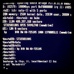
New 9front release "MOTHY MARTHA"
the changes from previous release include:
mothra improvements: fast scroll, text selection
updated manual pages
hjfs improvments and bugfixes
added "Rules of Acquisition" (/lib/roa)
devproc bugfixes
improved guesscpuhz()
fixed tftp lost ack packet bug
added eriks atazz and disk/smart
sata support for 4K sector drives


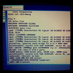
New 9front release "OFF KEY LEE"
changes include:
ACPI improvement (AliasOp AML instruction)
USB unassigned PciINTL work arround
Intel SCH busmastering dma support
mothra improvements (<script> tag, line break layout bugfix)
HTML support for lp
rio one line increment scroll (Shift)

People I work with recognize my computer easily: it's the one with nothing but yellow windows and blue bars on the screen. That's the text editor acme, written by Rob Pike for Plan 9 in the early 1990s. Acme focuses entirely on the idea of text as user interface. It's difficult to explain acme without seeing it, though, so I've put together a screencast explaining the basics of acme and showing a brief programming session. Remember as you watch the video that the 854x480 screen is quite cramped. Usually you'd run acme on a larger screen: even my MacBook Air has almost four times as much screen real estate.
The video doesn't show everything acme can do, nor does it show all the ways you can use it. Even small idioms like where you type text to be loaded or executed vary from user to user. To learn more about acme, read Rob Pike's paper “Acme: A User Interface for Programmers” and then try it.
Acme runs on most operating systems. If you use Plan 9 from Bell Labs, you already have it. If you use FreeBSD, Linux, OS X, or most other Unix clones, you can get it as part of Plan 9 from User Space. If you use Windows, I suggest trying acme as packaged in acme stand alone complex, which is based on the Inferno programming environment.
Mini-FAQ:
acme -f /mnt/font/Monaco/16a/font you get 16-point anti-aliased Monaco as your font, served via fontsrv. If you'd like to add X11 support to fontsrv, I'd be happy to apply the patch.
If you're interested in history, the predecessor to acme was called help. Rob Pike's paper “A Minimalist Global User Interface” describes it. See also “The Text Editor sam”
Correction: the smiley program in the video was written by Ken Thompson. I got it from Dennis Ritchie, the more meticulous archivist of the pair.
stanleylieber posted a photo:

New 9front "Robby Rubbish"
Changes include support for Intel 82567V ethernet and USB fixes for isochronous transfers (usb audio) and support for SK-8835 IBM Thinkpad USB Keyboard/Mice. date(1) got support to print ISO-8601 date and time and devshr now honors the noattach flag (RFNOMNT).


New 9front "Release Target Geronimo"
changes include:
aux/cpuid program to print Intel cpu features
netaudit program which checks network database for common mistakes
bugfixes for ndb/dns
fixed old RFNOMNT kernel bug
fix sleep / wakeup bug in devmnt and sdvirtio
pause function in games/gb
rio listing burried windows in button 3 menu
audiohda support for Intel SCH Pouslbo and Oaktrail
usb/kb support for Microsoft Sidewinder X5 Mouse
default configuration for 9bootpxe
tls support for sha256WithRSAEncryption (torproject.com)
bugfixes in jpg


New 9front release "Groovy Greg"
changes include:


New 9front release "Deaf Geoff"
this release consists mainly of bugfixes (cwfs, kfs, factotum, mothra) tho cdfs got updated from sources and sam undo command will jump to the change now (thanks aiju!) ;)


We should have some ways of coupling programs like garden hose--screw in another segment when it becomes necessary to massage data in another way. This is the way of IO also.That is the way of Go also. Go takes that idea and pushes it very far. It is a language of composition and coupling.
The range of abstractions that C++ can express elegantly, flexibly, and at zero costs compared to hand-crafted specialized code has greatly increased.That way of thinking just isn't the way Go operates. Zero cost isn't a goal, at least not zero CPU cost. Go's claim is that minimizing programmer effort is a more important consideration.


Last week, I gave a talk about Go at the Boston Google Developers Group meeting. There were some problems with the recording, so I have rerecorded the talk as a screencast and posted it on YouTube.
Here are the answers to questions asked at the end of the talk.
Q. How does Go work with debuggers?
To start, both Go toolchains include debugging information that gdb can read in the final binaries, so basic gdb functionality works on Go programs just as it does on C programs.
We’ve talked for a while about a custom Go debugger, but there isn’t one yet.
Many of the programs we want to debug are live, running programs. The net/http/pprof package provides debugging information like goroutine stacks, memory profiling, and cpu profiling in response to special HTTP requests.
Q. If a goroutine is stuck reading from a channel with no other references, does the goroutine get garbage collected?
No. From the garbage collection point of view, both sides of the channel are represented by the same pointer, so it can’t distinguish the receive and send sides. Even if we could detect this situation, we’ve found that it’s very useful to keep these goroutines around, because the program is probably heading for a deadlock. When a Go program deadlocks, it prints all its goroutine stacks and then exits. If we garbage collected the goroutines as they got stuck, the deadlock handler wouldn’t have anything useful to print except "your entire program has been garbage collected".
Q. Can a C++ program call into Go?
We wrote a tool called cgo so that Go programs can call into C, and we’ve implemented support for Go in SWIG, so that Go programs can call into C++. In those programs, the C or C++ can in turn call back into Go. But we don’t have support for a C or C++ program—one that starts execution in the C or C++ world instead of the Go world—to call into Go.
The hardest part of the cross-language calls is converting between the C calling convention and the Go calling convention, specifically with the regard to the implementation of segmented stacks. But that’s been done and works.
Making the assumption that these mixed-language binaries start in Go has simplified a number of parts of the implementation. I don’t anticipate any technical surprises involved in removing these assumptions. It’s just work.
Q. What are the areas that you specifically are trying to improve the language?
For the most part, I’m not trying to improve the language itself. Part of the effort in preparing Go 1 was to identify what we wanted to improve and do it. Many of the big changes were based on two or three years of experience writing Go programs, and they were changes we’d been putting off because we knew that they’d be disruptive. But now that Go 1 is out, we want to stop changing things and spend another few years using the language as it exists today. At this point we don’t have enough experience with Go 1 to know what really needs improvement.
My Go work is a small amount of fixing bugs in the libraries or in the compiler and a little bit more work trying to improve the performance of what’s already there.
Q. What about talking to databases and web services?
For databases, one of the packages we added in Go 1 is a standard database/sql package. That package defines a standard API for interacting with SQL databases, and then people can implement drivers that connect the API to specific database implementations like SQLite or MySQL or Postgres.
For web services, you’ve seen the support for JSON and XML encodings. Those are typically good enough for ad hoc REST services. I recently wrote a package for connecting to the SmugMug photo hosting API, and there’s one generic call that unmarshals the response into a struct of the appropriate type, using json.Unmarshal. I expect that XML-based web services like SOAP could be framed this way too, but I’m not aware of anyone who’s done that.
Inside Google, of course, we have plenty of services, but they’re based on protocol buffers, so of course there’s a good protocol buffer library for Go.
Q. What about generics? How far off are they?
People have asked us about generics from day 1. The answer has always been, and still is, that it’s something we’ve put a lot of thought into, but we haven’t yet found an approach that we think is a good fit for Go. We’ve talked to people who have been involved in the design of generics in other languages, and they’ve almost universally cautioned us not to rush into something unless we understand it very well and are comfortable with the implications. We don’t want to do something that we’ll be stuck with forever and regret.
Also, speaking for myself, I don’t miss generics when I write Go programs. What’s there, having built-in support for arrays, slices, and maps, seems to work very well.
Finally, we just made this promise about backwards compatibility with the release of Go 1. If we did add some form of generics, my guess is that some of the existing APIs would need to change, which can’t happen until Go 2, which I think is probably years away.
Q. What types of projects does Google use Go for?
Most of the things we use Go for I can’t talk about. One notable exception is that Go is an App Engine language, which we announced at I/O last year. Another is vtocc, a MySQL load balancer used to manage database lookups in YouTube’s core infrastructure.
Q. How does the Plan 9 toolchain differ from other compilers?
It’s a completely incompatible toolchain in every way. The main difference is that object files don’t contain machine code in the sense of having the actual instruction bytes that will be used in the final binary. Instead they contain a custom encoding of the assembly listings, and the linker is in charge of turning those into actual machine instructions. This means that the assembler, C compiler, and Go compiler don’t all duplicate this logic. The main change for Go is the support for segmented stacks.
I should add that we love the fact that we have two completely different compilers, because it keeps us honest about really implementing the spec.
Q. What are segmented stacks?
One of the problems in threaded C programs is deciding how big a stack each thread should have. If the stack is too small, then the thread might run out of stack and cause a crash or silent memory corruption, and if the stack is too big, then you’re wasting memory. In Go, each goroutine starts with a small stack, typically 4 kB, and then each function checks if it is about to run out of stack and if so allocates a new stack segment that gets recycled once it’s not needed anymore.
Gccgo supports segmented stacks, but it requires support added recently to the new GNU linker, gold, and that support is only implemented for x86-32 and x86-64.
Segmented stacks are something that lots of people have done before in experimental or research systems, but they have never made it into the C toolchains.
Q. What is the overhead of segmented stacks?
It’s a few instructions per function call. It’s been a long time since I tried to measure the precise overhead, but in most programs I expect it to be not more than 1-2%. There are definitely things we could do to try to reduce that, but it hasn’t been a concern.
Q. Do goroutine stacks adapt in size?
The initial stack allocated for a goroutine does not adapt. It’s always 4k right now. It has been other values in the past but always a constant. One of the things I’d like to do is to look at what the goroutine will be running and adjust the stack accordingly, but I haven’t.
Q. Are there any short-term plans for dynamic loading of modules?
No. I don’t think there are any technical surprises, but assuming that everything is statically linked simplified some of the implementation. Like with calling Go from C++ programs, I believe it’s just work.
Gccgo might be closer to support for this, but I don’t believe that it supports dynamic loading right now either.
Q. How much does the language spec say about reflection?
The spec is intentionally vague about reflection, but package reflect’s API is definitely part of the Go 1 definition. Any conforming implementation would need to implement that API. In fact, gc and gccgo do have different implementations of that package reflect API, but then the packages that use reflect like fmt and json can be shared.
Q. Do you have a release schedule?
We don’t have any fixed release schedule. We’re not keeping things secret, but we’re also not making commitments to specific timelines.
Go 1 was in progress publicly for months, and if you watched you could see the bug count go down and the release candidates announced, and so on.
Right now we’re trying to slow down. We want people to write things using Go, which means we need to make it a stable foundation to build on. Go 1.0.1, the first bug release, was released four weeks after Go 1, and Go 1.0.2 was seven weeks after Go 1.0.1.
Q. Where do you see Go in five years? What languages will it replace?
I hope that it will still be at golang.org, that the Go project will still be thriving and relevant. We built it to write the kinds of programs we’ve been writing in C++, Java, and Python, but we’re not trying to go head-to-head with those languages. Each of those has definite strengths that make them the right choice for certain situations. We think that there are plenty of situations, though, where Go is a better choice.
If Go doesn’t work out, and for some reason in five years we’re programming in something else, I hope the something else would have the features I talked about, specifically the Go way of doing interfaces and the Go way of handling concurrency.
If Go fails but some other language with those two features has taken over the programming landscape, if we can move the computing world to a language with those two features, then I’d be sad about Go but happy to have gotten to that situation.
Q. What are the limits to scalability with building a system with many goroutines?
The primary limit is the memory for the goroutines. Each goroutine starts with a 4kB stack and a little more per-goroutine data, so the overhead is between 4kB and 5kB. That means on this laptop I can easily run 100,000 goroutines, in 500 MB of memory, but a million goroutines is probably too much.
For a lot of simple goroutines, the 4 kB stack is probably more than necessary. If we worked on getting that down we might be able to handle even more goroutines. But remember that this is in contrast to C threads, where 64 kB is a tiny stack and 1-4MB is more common.
Q. How would you build a traditional barrier using channels?
It’s important to note that channels don’t attempt to be a concurrency Swiss army knife. Sometimes you do need other concepts, and the standard sync package has some helpers. I’d probably use a sync.WaitGroup.
If I had to use channels, I would do it like in the web crawler example, with a channel that all the goroutines write to, and a coordinator that knows how many responses it expects.
Q. What is an example of the kind of application you’re working on performance for? How will you beat C++?
I haven’t been focusing on specific applications. Go is still young enough that if you run some microbenchmarks you can usually find something to optimize. For example, I just sped up floating point computation by about 25% a few weeks ago. I’m also working on more sophisticated analyses for things like escape analysis and bounds check elimination, which address problems that are unique to Go, or at least not problems that C++ faces.
Our goal is definitely not to beat C++ on performance. The goal for Go is to be near C++ in terms of performance but at the same time be a much more productive environment and language, so that you’d rather program in Go.
Q. What are the security features of Go?
Go is a type-safe and memory-safe language. There are no dangling pointers, no pointer arithmetic, no use-after-free errors, and so on.
You can break the rules by importing package unsafe, which gives you a special type unsafe.Pointer. You can convert any pointer or integer to an unsafe.Pointer and back. That’s the escape hatch, which you need sometimes, like for extracting the bits of a float64 as a uint64. But putting it in its own package means that unsafe code is explicitly marked as unsafe. If your program breaks in a strange way, you know where to look.
Isolating this power also means that you can restrict it. On App Engine you can’t import package unsafe in the code you upload for your app.
I should point out that the current Go implementation does have data races, but they are not fundamental to the language. It would be possible to eliminate the races at some cost in efficiency, and for now we’ve decided not to do that. There are also tools such as Thread Sanitizer that help find these kinds of data races in Go programs.
Q. What language do you think Go is trying to displace?
I don’t think of Go that way. We were writing C++ code before we did Go, so we definitely wanted not to write C++ code anymore. But we’re not trying to displace all C++ code, or all Python code, or all Java code, except maybe in our own day-to-day work.
One of the surprises for me has been the variety of languages that new Go programmers used to use. When we launched, we were trying to explain Go to C++ programmers, but many of the programmers Go has attracted have come from more dynamic languages like Python or Ruby.
Q. How does Go make it possible to use multiple cores?
Go lets you tell the runtime how many operating system threads to use for executing goroutines, and then it muxes the goroutines onto those threads. So if you’ve written a program that has four or more goroutines executing simultaneously, you can tell the runtime to use four OS threads and then you’re running on four cores.
We’ve been pleasantly surprised by how easy people find it to write these kinds of programs. People who have not written parallel or concurrent programs before write concurrent Go programs using channels that can take advantage of multiple cores, and they enjoy the experience. That’s more than you can usually say for C threads. Joe Armstrong, one of the creators of Erlang, makes the point that thinking about concurrency in terms of communication might be more natural for people, since communication is something we’ve done for a long time. I agree.
Q. How does the muxing of goroutines work?
It’s not very smart. It’s the simplest thing that isn’t completely stupid: all the scheduling operations are O(1), and so on, but there’s a shared run queue that the various threads pull from. There’s no affinity between goroutines and threads, there’s no attempt to make sophisticated scheduling decisions, and there’s not even preemption.
The goroutine scheduler was the first thing I wrote when I started working on Go, even before I was working full time on it, so it’s just about four years old. It has served us surprisingly well, but we’ll probably want to replace it in the next year or so. We’ve been having some discussions recently about what we’d want to try in a new scheduler.
Q. Is there any plan to bootstrap Go in Go, to write the Go compiler in Go?
There’s no immediate plan. Go does ship with a Go program parser written in Go, so the first piece is already done, and there’s an experimental type checker in the works, but those are mainly for writing program analysis tools. I think that Go would be a great language to write a compiler in, but there’s no immediate plan. The current compiler, written in C, works well.
I’ve worked on bootstrapped languages in the past, and I found that bootstrapping is not necessarily a good fit for languages that are changing frequently. It reminded me of climbing a cliff and screwing hooks into the cliff once in a while to catch you if you fall. Once or twice I got into situations where I had identified a bug in the compiler, but then trying to write the code to fix the bug tickled the bug, so it couldn’t be compiled. And then you have to think hard about how to write the fix in a way that avoids the bug, or else go back through your version control history to find a way to replay history without introducing the bug. It’s not fun.
The fact that Go wasn’t written in itself also made it much easier to make significant language changes. Before the initial release we went through a handful of wholesale syntax upheavals, and I’m glad we didn’t have to worry about how we were going to rebootstrap the compiler or ensure some kind of backwards compatibility during those changes.
Finally, I hope you’ve read Ken Thompson’s Turing Award lecture, Reflections on Trusting Trust. When we were planning the initial open source release, we liked to joke that no one in their right mind would accept a bootstrapped compiler binary written by Ken.
Q. What does Go do to compile efficiently at scale?
This is something that we talked about a lot in early talks about Go. The main thing is that it cuts off transitive dependencies when compiling a single module. In most languages, if package A imports B, and package B imports C, then the compilation of A reads not just the compiled form of B but also the compiled form of C. In large systems, this gets out of hand quickly. For example, in C++ on my Mac, including <iostream> reads 25,326 lines from 131 files. (C and C++ headers aren't “compiled form,” but the problem is the same.) Go promises that each import reads a single compiled package file. If you need to know something about other packages to understand that package’s API, then the compiled file includes the extra information you need, but only that.
Of course, if you are building from scratch and package A imports B which imports C, then of course C has to be compiled first, and then B, and then A. The import point is that when you go to compile A, you don’t reload C’s object file. In a real program, the dependencies are usually not a chain like this. We might have A1, A2, A3, and so on all importing B. It’s a significant win if none of them need to reread C.
Q. How do you identify a good project for Go?
I think a good project for Go is one that you’re excited about writing in Go. Go really is a general purpose programming language, and except for the compiler work, it’s the only language I’ve written significant programs in for the past four years.
Most of the people I know who are using Go are using it for networked servers, where the concurrency features have something contribute, but it’s great for other contexts too. I’ve used it to write a simple mail reader, file system implementations to read old disks, and a variety of other unnetworked programs.
Q. What is the current and future IDE support for Go?
I’m not an IDE user in the modern sense, so really I don’t know. We think that it would be possible to write a really nice IDE specifically for Go, but it’s not something we’ve had time to explore. The Go distribution has a misc directory that contains basic Go support for common editors, and there is a Goclipse project to write an Eclipse-based IDE, but I don’t know much about those.
The development environment I use, acme, is great for writing Go code, but not because of any custom Go support.
If you have more questions, please consult these resources.

stanleylieber posted a photo:
stanleylieber posted a photo:
stanleylieber posted a photo:

stanleylieber posted a photo:
stanleylieber posted a photo:
stanleylieber posted a photo:
stanleylieber posted a photo:
stanleylieber posted a photo:
stanleylieber posted a photo:

stanleylieber posted a photo:
stanleylieber posted a photo:
stanleylieber posted a photo:
stanleylieber posted a photo:

stanleylieber posted a photo:

stanleylieber posted a photo:

stanleylieber posted a photo:

stanleylieber posted a photo:

stanleylieber posted a photo:

stanleylieber posted a photo:

stanleylieber posted a photo:

QR codes are 2-dimensional bar codes that encode arbitrary text strings. A common use of QR codes is to encode URLs so that people can scan a QR code (for example, on an advertising poster, building roof, volleyball bikini, belt buckle, or airplane banner) to load a web site on a cell phone instead of having to “type” in a URL.
QR codes are encoded using Reed-Solomon error-correcting codes, so that a QR scanner does not have to see every pixel correctly in order to decode the content. The error correction makes it possible to introduce a few errors (fewer than the maximum that the algorithm can fix) in order to make an image. For example, in 2008, Duncan Robertson took a QR code for “http://bbc.co.uk/programmes” (left) and introduced errors in the form of a BBC logo (right):

That's a neat trick and a pretty logo, but it's uninteresting from a technical standpoint. Although the BBC logo pixels look like QR code pixels, they are not contribuing to the QR code. The QR reader can't tell much difference between the BBC logo and the Union Jack. There's just a bunch of noise in the middle either way.

Since the BBC QR logo appeared, there have been many imitators. Most just slap an obviously out-of-place logo in the middle of the code. This Disney poster is notable for being more in the spirit of the BBC code.
There's a different way to put pictures in QR codes. Instead of scribbling on redundant pieces and relying on error correction to preserve the meaning, we can engineer the encoded values to create the picture in a code with no inherent errors, like these:


This post explains the math behind making codes like these, which I call QArt codes. I have published the Go programs that generated these codes at code.google.com/p/rsc and created a web site for creating these codes.
For error correction, QR uses Reed-Solomon coding (like nearly everything else). For our purposes, Reed-Solomon coding has two important properties. First, it is what coding theorists call a systematic code: you can see the original message in the encoding. That is, the Reed-Solomon encoding of “hello” is “hello” followed by some error-correction bytes. Second, Reed-Solomon encoded messages can be XOR'ed: if we have two different Reed-Solomon encoded blocks b1 and b2 corresponding to messages m1 and m2, b1 ⊕ b2 is also a Reed-Solomon encoded block; it corresponds to the message m1 ⊕ m2. (Here, ⊕ means XOR.) If you are curious about why these two properties are true, see my earlier post, Finite Field Arithmetic and Reed-Solomon Coding.
A QR code has a distinctive frame that help both people and computers recognize them as QR codes. The details of the frame depend on the exact size of the code—bigger codes have room for more bits—but you know one when you see it: the outlined squares are the giveaway. Here are QR frames for a sampling of sizes:
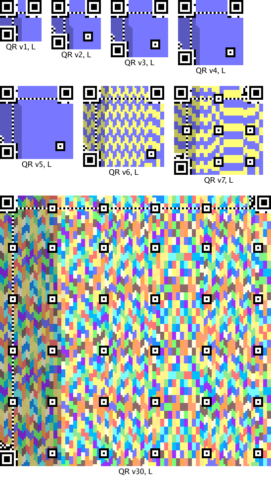
The colored pixels are where the Reed-Solomon-encoded data bits go. Each code may have one or more Reed-Solomon blocks, depending on its size and the error correction level. The pictures show the bits from each block in a different color. The L encoding is the lowest amount of redundancy, about 20%. The other three encodings increase the redundancy, using 38%, 55%, and 65%.
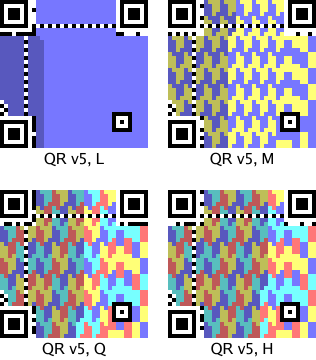
(By the way, you can read the redundancy level from the top pixels in the two leftmost columns. If black=0 and white=1, then you can see that 00 is L, 01 is M, 10 is Q, and 11 is H. Thus, you can tell that the QR code on the T-shirt in this picture is encoded at the highest redundancy level, while this shirt uses the lowest level and therefore might take longer or be harder to scan.
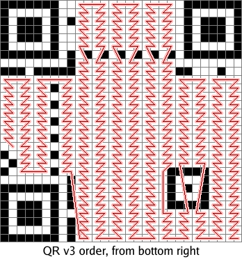
As I mentioned above, the original message bits are included directly in the message's Reed-Solomon encoding. Thus, each bit in the original message corresponds to a pixel in the QR code. Those are the lighter pixels in the pictures above. The darker pixels are the error correction bits. The encoded bits are laid down in a vertical boustrophedon pattern in which each line is two columns wide, starting at the bottom right corner and ending on the left side:
We can easily work out where each message bit ends up in the QR code. By changing those bits of the message, we can change those pixels and draw a picture. There are, however, a few complications that make things interesting.
The first complication is that the encoded data is XOR'ed with an obfuscating mask to create the final code. There are eight masks:
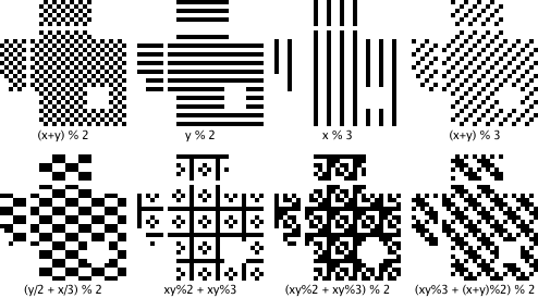
An encoder is supposed to choose the mask that best hides any patterns in the data, to keep those patterns from being mistaken for framing boxes. In our encoder, however, we can choose a mask before choosing the data. This violates the spirit of the spec but still produces legitimate codes.
The second complication is that we want the QR code's message to be intelligible. We could draw arbitrary pictures using arbitrary 8-bit data, but when scanned the codes would produce binary garbage. We need to limit ourselves to data that produces sensible messages. Luckily for us, QR codes allow messages to be written using a few different alphabets. One alphabet is 8-bit data, which would require binary garbage to draw a picture. Another is numeric data, in which every run of 10 bits defines 3 decimal digits. That limits our choice of pixels slightly: we must not generate a 10-bit run with a value above 999. That's not complete flexibility, but it's close: 9.96 bits of freedom out of 10. If, after encoding an image, we find that we've generated an invalid number, we pick one of the 5 most significant bits at random—all of them must be 1s to make an invalid number—hard wire that bit to zero, and start over.
Having only decimal messages would still not be very interesting: the message would be a very large number. Luckily for us (again), QR codes allow a single message to be composed from pieces using different encodings. The codes I have generated consist of an 8-bit-encoded URL ending in a # followed by a numeric-encoded number that draws the actual picture:
The leading URL is the first data encoded; it takes up the right side of the QR code. The error correction bits take up the left side.
When the phone scans the QR code, it sees a URL; loading it in a browser visits the base page and then looks for an internal anchor on the page with the given number. The browser won't find such an anchor, but it also won't complain.
The techniques so far let us draw codes like this one:


The second copy darkens the pixels that we have no control over: the error correction bits on the left and the URL prefix on the right. I appreciate the cyborg effect of Peter melting into the binary noise, but it would be nice to widen our canvas.
The third complication, then, is that we want to draw using more than just the slice of data pixels in the middle of the image. Luckily, we can.
I mentioned above that Reed-Solomon messages can be XOR'ed: if we have two different Reed-Solomon encoded blocks b1 and b2 corresponding to messages m1 and m2, b1 ⊕ b2 is also a Reed-Solomon encoded block; it corresponds to the message m1 ⊕ m2. (In the notation of the previous post, this happens because Reed-Solomon blocks correspond 1:1 with multiples of g(x). Since b1 and b2 are multiples of g(x), their sum is a multiple of g(x) too.) This property means that we can build up a valid Reed-Solomon block from other Reed-Solomon blocks. In particular, we can construct the sequence of blocks b0, b1, b2, ..., where bi is the block whose data bits are all zeros except for bit i and whose error correction bits are then set to correspond to a valid Reed-Solomon block. That set is a basis for the entire vector space of valid Reed-Solomon blocks. Here is the basis matrix for the space of blocks with 2 data bytes and 2 checksum bytes:
| 1 | 1 | 1 | 1 | 1 | 1 | 1 | 1 | 1 | 1 | ||||||||||||||||||||||
| 1 | 1 | 1 | 1 | 1 | 1 | 1 | 1 | 1 | 1 | 1 | 1 | ||||||||||||||||||||
| 1 | 1 | 1 | 1 | 1 | 1 | ||||||||||||||||||||||||||
| 1 | 1 | 1 | 1 | 1 | 1 | ||||||||||||||||||||||||||
| 1 | 1 | 1 | 1 | 1 | 1 | ||||||||||||||||||||||||||
| 1 | 1 | 1 | 1 | 1 | 1 | ||||||||||||||||||||||||||
| 1 | 1 | 1 | 1 | 1 | 1 | ||||||||||||||||||||||||||
| 1 | 1 | 1 | 1 | 1 | 1 | ||||||||||||||||||||||||||
| 1 | 1 | 1 | 1 | 1 | 1 | 1 | 1 | 1 | 1 | ||||||||||||||||||||||
| 1 | 1 | 1 | 1 | ||||||||||||||||||||||||||||
| 1 | 1 | 1 | 1 | ||||||||||||||||||||||||||||
| 1 | 1 | 1 | 1 | ||||||||||||||||||||||||||||
| 1 | 1 | 1 | 1 | ||||||||||||||||||||||||||||
| 1 | 1 | 1 | 1 | ||||||||||||||||||||||||||||
| 1 | 1 | 1 | 1 | ||||||||||||||||||||||||||||
| 1 | 1 | 1 | 1 | ||||||||||||||||||||||||||||
The missing entries are zeros. The gray columns highlight the pixels we have complete control over: there is only one row with a 1 for each of those pixels. Each time we want to change such a pixel, we can XOR our current data with its row to change that pixel, not change any of the other controlled pixels, and keep the error correction bits up to date.
So what, you say. We're still just twiddling data bits. The canvas is the same.
But wait, there's more! The basis we had above lets us change individual data pixels, but we can XOR rows together to create other basis matrices that trade data bits for error correction bits. No matter what, we're not going to increase our flexibility—the number of pixels we have direct control over cannot increase—but we can redistribute that flexibility throughout the image, at the same time smearing the uncooperative noise pixels evenly all over the canvas. This is the same procedure as Gauss-Jordan elimination, the way you turn a matrix into row-reduced echelon form.
This matrix shows the result of trying to assert control over alternating pixels (the gray columns):
| 1 | 1 | 1 | 1 | 1 | 1 | 1 | 1 | 1 | 1 | ||||||||||||||||||||||
| 1 | 1 | 1 | 1 | 1 | 1 | 1 | 1 | 1 | 1 | ||||||||||||||||||||||
| 1 | 1 | 1 | 1 | 1 | 1 | ||||||||||||||||||||||||||
| 1 | 1 | 1 | 1 | 1 | 1 | ||||||||||||||||||||||||||
| 1 | 1 | 1 | 1 | ||||||||||||||||||||||||||||
| 1 | 1 | 1 | 1 | 1 | 1 | ||||||||||||||||||||||||||
| 1 | 1 | 1 | 1 | 1 | 1 | ||||||||||||||||||||||||||
| 1 | 1 | 1 | 1 | ||||||||||||||||||||||||||||
| 1 | 1 | 1 | 1 | 1 | 1 | 1 | 1 | 1 | 1 | ||||||||||||||||||||||
| 1 | 1 | 1 | 1 | ||||||||||||||||||||||||||||
| 1 | 1 | 1 | 1 | ||||||||||||||||||||||||||||
| 1 | 1 | 1 | 1 | 1 | 1 | ||||||||||||||||||||||||||
| 1 | 1 | 1 | 1 | 1 | 1 | 1 | 1 | ||||||||||||||||||||||||
| 1 | 1 | 1 | 1 | ||||||||||||||||||||||||||||
| 1 | 1 | 1 | 1 | ||||||||||||||||||||||||||||
| 1 | 1 | 1 | 1 | ||||||||||||||||||||||||||||
The matrix illustrates an important point about this trick: it's not completely general. The data bits are linearly independent, but there are dependencies between the error correction bits that mean we often can't have every pixel we ask for. In this example, the last four pixels we tried to get were unavailable: our manipulations of the rows to isolate the first four error correction bits zeroed out the last four that we wanted.
In practice, a good approach is to create a list of all the pixels in the Reed-Solomon block sorted by how useful it would be to be able to set that pixel. (Pixels from high-contrast regions of the image are less important than pixels from low-contrast regions.) Then, we can consider each pixel in turn, and if the basis matrix allows it, isolate that pixel. If not, no big deal, we move on to the next pixel.
Applying this insight, we can build wider but noisier pictures in our QR codes:


The pixels in Peter's forehead and on his right side have been sacrificed for the ability to draw the full width of the picture.
We can also choose the pixels we want to control at random, to make Peter peek out from behind a binary fog:


One final trick. QR codes have no required orientation. The URL base pixels that we have no control over are on the right side in the canonical orientation, but we can rotate the QR code to move them to other edges.


All the source code for this post, including the web server, is at code.google.com/p/rsc/source/browse/qr. If you liked this, you might also like Zip Files All The Way Down.
Alex Healy pointed out that valid Reed-Solomon encodings are closed under XOR, which is the key to spreading the picture into the error correction pixels. Peter Weinberger has been nothing but gracious about the overuse of his binary likeness. Thanks to both.
Finite fields are a branch of algebra formally defined in the 1820s, but interest in the topic can be traced back to public sixteenth-century polynomial-solving contests. For the next few centuries, finite fields had little practical value, but all changed in the last fifty years. It turns out that they are useful for many applications in modern computing, such as encryption, data compression, and error correction.
In particular, Reed-Solomon codes are an error-correcting code based on finite fields and used everywhere today. One early significant use was in the Voyager spacecraft: the messages it still sends back today, from the edge of the solar system, are heavily Reed-Solomon encoded so that even if only a small fragment makes it back to Earth, we can still reconstruct the message. Reed-Solomon coding is also used on CDs to withstand scratches, in wireless communications to withstand transmission problems, in QR codes to withstand scanning errors or smudges, in disks to withstand loss of fragments of the media, in high-level storage systems like Google's GFS and BigTable to withstand data loss and also to reduce read latency (the read can complete without waiting for all the responses to arrive).
This post shows how to implement finite field arithmetic efficiently on a computer, and then how to use that to implement Reed-Solomon encoding.
One way mathematicians study numbers is to abstract away the numbers themselves and focus on the operations. (This is kind of an object-oriented approach to math.) A field is defined as a set F and operators + and · on elements of F that satisfy the following properties:
You probably recognize those properties from high school algebra class: the most well-known example of a field is the real numbers, where + is addition and · is multiplication. Other examples are complex numbers and fractions.
A mathematician doesn't have to prove the same results over and over
for the real numbers ℝ, the complex numbers ℂ, the fractions ℚ, and so on.
Instead, she can prove that a particular result holds for all fields—by assuming only
the above properties, called the field axioms. Then she can apply the result by
substituting a specific instance like the real numbers for the general idea of a field,
the same way that a programmer can implement just one vector(T)
and then instantiate it as vector(int), vector(string) and so on.
The integers ℤ are not a field: they lack multiplicative inverses. For example, there is no number that you can multiply by 2 to get 1, no 1/2. Surprisingly, though, the integers modulo any prime p do form a field. For example, the integers modulo 5 are 0, 1, 2, 3, 4. 1+4 = 0 (mod 5), so we say that 4 = −1. Similarly, 2·3 = 1 (mod 5), so we say that 3 = 1/2. After we've proved that ℤ/p is in fact a field, all the results about fields can be applied to ℤ/p. This is very useful: it lets us apply our intuition about the very familiar real numbers to these less familiar numbers. This field is written ℤ/p to emphasize that we're dealing with what's left after subtracting out all the p's. That is, we're dealing with what's left if you assume that p = 0. When you make that assumption, you get math that wraps around at p. These fields are called finite fields because, in contrast to fields like the real numbers, they have a finite number of elements.
For a programmer, the most interesting finite field is
ℤ/2, which contains just the integers 0, 1. Addition
is the same as XOR, and multiplication is the same as AND.
Note that ℤ/p is only a field when p is prime:
arithmetic on uint8 variables corresponds
to ℤ/256, but it is not a field: there is no 1/2.
The only problem with fields is that there's not a ton you can do with just the field axioms. One thing you can do is build polynomials, which were the original motivation for the mathematicians who pioneered the use of fields in the early 1800s. If we introduce a symbolic variable x, then we can build polynomials whose coefficients are field values. We'll write F[x] to denote the polynomials over x using coefficients from F. For example, if we use the real numbers ℝ as our field, then the polynomials ℝ[x] include x2+1, x+2, and 3.14x2 − 2.72x + 1.41. Like integers, these polynomials can be added and multiplied, but not always divided—what is (x2+1)/(x+2)?—so they are not a field. However, remember how the integers are not a field but the integers modulo a prime are a field? The same happens here: polynomials are not a field but polynomials modulo some prime polynomial are.
What does “polynomials modulo some prime polynomial” mean anyway? A prime polynomial is one that cannot be factored, like x2+1 cannot be factored using real numbers. The field ℤ/5 is what you get by doing math under the assumption that 5 = 0; similarly, ℝ[x]/(x2+1) is what you get by doing math under the assumption that x2+1 = 0. Just as ℤ/5 math never deals with numbers as big as 5, ℝ[x]/(x2+1) math never deals with polynomials as big as x2: anything bigger can have some multiple of x2+1 subtracted out again. That is, the polynomials in ℝ[x]/(x2+1) are bounded in size: they have only x1 and x0 (constant) terms. To add polynomials, we just add the coefficients using the addition rule from the coefficient's field, independently, like a vector addition. To multiply polynomials, we have to do the multiplication and then subtract out any x2+1 we can. If we have (ax+b)·(cx+d), we can expand this to (a·c)x2 + (b·c+a·d)x + (b·d), and then subtract (a·c)(x2+1) = (a·c)x2 + (a·c), producing the final result: (b·c+a·d)x + (b·d−a·c). That might seem like a funny definition of multiplication, but it does in fact obey the field axioms. In fact, this particular field is more familiar than it looks: it is the complex numbers ℂ, but we've written x instead of the usual i. Assuming that x2+1 = 0 is, except for a renaming, the same as defining i2 = −1.
Doing all our math modulo a prime polynomial let us take the field of real numbers and produce a field whose elements are pairs of real numbers. We can apply the same trick to take a finite field like ℤ/p and product a field whose elements are fixed-length vectors of elements of ℤ/p. The original ℤ/p has p elements. If we construct (ℤ/p)[x]/f(x), where f(x) is a prime polynomial of degree n (f's maximum x exponent is n), the resulting field has pn elements: all the vectors made up of n elements from ℤ/p. Incredibly, the choice of prime polynomial doesn't matter very much: any two finite fields of size pn have identical structure, even if they give the individual elements different names. Because of this, it makes sense to refer to all the finite fields of size pn as one concept: GF(pn). The GF stands for Galois Field, in honor of Évariste Galois, who was the first to study these. The exact polynomial chosen to produce a particular GF(pn) is an implementation detail.
For a programmer, the most interesting finite fields constructed this way are GF(2n)—the polynomial extensions of ℤ/2—because the elements of GF(2n) are bit vectors of length n. As a concrete example, consider (ℤ/2)[x]/(x8+x4+x3+x+1) . The field has 28 elements: each can be represented by a single byte. The byte with binary digits b7b6b5b4b3b2b1b0 represents the polynomial b7·x7 + b6·x6 + b5·x5 + b4·x4 + b3·x3 + b2·x2 + b1·x1 + b0. To add polynomials, we add coefficients. Since the coefficients are from ℤ/2, adding coefficients means XOR'ing each bit position separately, which is something computer hardware can do easily. Multiplying the polynomials is more difficult, because standard multiplication hardware is based on adding, but we need a multiplication based on XOR'ing. Because the coefficient math wraps at 2, (x2+x)·(x+1) = x3+2x2+x = x3+x, while computer multiplication would choose 1102* 0112 = 6 * 3 = 18 = 100102. However, it turns out that we can implement this field multiplication with a simple lookup table. In a finite field, there is always at least one element α that can serve as a generator. All the other non-zero elements are powers of α: α, α2, α3, and so on. This α is not symbolic like x: it's a specific element. For example, in ℤ/5, we can use α=2: {α, α2, α3, α4} = {2, 4, 8, 16} = {2, 4, 3, 1}. In GF(2n) the math is more complex but still works. If we know the generator, then we can, by repeated multiplication, create a lookup table exp[i] = αⁱ and an inverse table log[αⁱ] = i. Multiplication is then just a few table lookups: assuming a and b are non-zero, a·b = exp[log[a]+log[b]]. (That's a normal integer +, to add the exponents, not an XOR.)
The fact that GF(2n) can be implemented efficiently on a computer means that we can implement systems based on mathematical theorems without worrying about the usual overflow problems you get when modeling integers or real numbers. To be sure, GF(2n) behaves quite differently from the integers in many ways, but if all you need is the field axioms, it's good enough, and it eliminates any need to worry about overflow or arbitrary precision calculations. Because of the lookup table, GF(28) is by far the most common choice of field in a computer algorithm. For example, the Advanced Encryption Standard (AES, formerly Rijndael) is built around GF(28) arithmetic, as are nearly all implementations of Reed-Solomon coding.
Let's begin by defining a Field type that will
represent the specific instance of GF(28) defined by a
given polynomial.
The polynomial must be of degree 8, meaning that
its binary representation has the 0x100 bit set and no
higher bits set.
type Field struct {
    ...
}
Addition is just XOR, no matter what the polynomial is:
// Add returns the sum of x and y in the field.
func (f *Field) Add(x, y byte) byte {
    return x ^ y
}
Multiplication is where things get interesting. If you'd used binary (and Go) in grade school, you might have learned this algorithm for multiplying two numbers (this is not finite field arithmetic):
// Grade-school multiplication in binary: mul returns the product x×y.
func mul(x, y int) int {
    z := 0
    for x > 0 {
        if x&1 != 0 {
            z += y
        }
        x >>= 1
        y <<= 1
    }
    return z
}
The running total z accumulates the product of x and y.
The first iteration of this loop adds y to z if the
low bit (the 1s digit) of x is 1.
The next iteration adds y*2 if the next bit (the 2s digit, now shifted down) of
x is 1.
The next iteration adds y*4 if the 4s digit is 1, and so on.
Each iteration shifts x to the right to chop off the processed digit
and shifts y to the left to multiply by two.
To adapt this to multiply in a finite field, we need to make two changes.
First, addition is XOR, so we use ^= instead of +=
to add to z.
Second, we need to make the multiply reduce modulo the polynomial.
Assuming that the inputs have already been reduced, the only chance
of exceeding the polynomial comes from the shift of y.
After the shift, then, we can check to see if we've overflowed, and if so,
subtract (XOR) out one copy of the polynomial.
The finite field version, then, is:
// GF(256) mutiplication: mul returns the product x×y mod poly.
func mul(x, y, poly int) int {
    z := 0
    for x > 0 {
        if x&1 != 0 {
            z ^= y
        }
        x >>= 1
        y <<= 1
        if y&0x100 != 0 {
            y ^= poly
        }
    }
    return z
}
We might want to do a lot of multiplication, though,
and this loop is too slow. There aren't that many inputs—only 28×28 of them—so one
option is to build a 64kB lookup table. With some cleverness, we can
build a smaller lookup table.
In the NewField
constructor, we can compute α0, α1, α2, ..., record the sequence
in an exp array, and record the inverse in
a log array.
Then we can reduce multiplication to addition of logarithms,
like a slide rule does.
// A Field represents an instance of GF(256) defined by a specific polynomial.
type Field struct {
    log [256]byte // log[0] is unused
    exp [510]byte
}

// NewField returns a new field corresponding to
// the given polynomial and generator.
func NewField(poly, α int) *Field {
    var f Field
    x := 1
    for i := 0; i < 255; i++ {
        f.exp[i] = byte(x)
        f.exp[i+255] = byte(x)
        f.log[x] = byte(i)
        x = mul(x, α, poly)
    }
    f.log[0] = 255
    return &f
}
The values of the exp function cycle with period 255
(not 256, because 0 is impossible): α255 = 1.
The straightforward way to implement Exp, then,
is to look up the entry given by the exponent modulo 255.
// Exp returns the base 2 exponential of e in the field.
// If e < 0, Exp returns 0.
func (f *Field) Exp(e int) byte {
    if e < 0 {
        return 0
    }
    return f.exp[e%255]
}
Log is an even simpler table lookup, because the input
is only a byte:
// Log returns the base 2 logarithm of x in the field.
// If x == 0, Log returns -1.
func (f *Field) Log(x byte) int {
    if x == 0 {
        return -1
    }
    return int(f.log[x])
}
Mul is where things get interesting.
The obvious implementation of Mul is exp[(log[x]+log[y])%255],
but if we double the exp array, so that it is 510 elements long,
we can drop the relatively expensive %255:
// Mul returns the product of x and y in the field.
func (f *Field) Mul(x, y byte) byte {
    if x == 0 || y == 0 {
        return 0
    }
    return f.exp[int(f.log[x])+int(f.log[y])]
}
Inv returns the multiplicative inverse, 1/x.
We don't implement divide: instead of x/y, we can use x · 1/y.
// Inv returns the multiplicative inverse of x in the field.
// If x == 0, Inv returns 0.
func (f *Field) Inv(x byte) byte {
    if x == 0 {
        return 0
    }
    return f.exp[255-f.log[x]]
}
In 1960, Irving Reed and Gustave Solomon proposed a way to build an error-correcting code using GF(2n). The method interpreted the m message bits as coefficients of a polynomial f of degree m−1 over GF(2n) and then sent f(0), f(α), f(α2), f(α3), ..., f(1). Any m of these, if received correctly, suffice to reconstruct f, and then the message can be read off the coefficients. To find a correct set, Reed and Solomon's algorithm constructed the f corresponding to every possible subset of m received values and then chose the most common one in a majority vote. As long as no more than (2n−m)/2 values were corrupted in transit, the majority will agree on the correct value of f. This decoding algorithm is very expensive, too expensive for long messages. As a result, the Reed-Solomon approach sat unused for almost a decade. In 1969, however, Elwyn Berlekamp and James Massey proposed a variant with an efficient decoding algorithm. In the 1980s, Berlekamp and Lloyd Welch developed an even more efficient decoding algorithm that is the one typically used today. These decoding algorithms are based on systems of equations far too complex to explain here; in this post, we will only deal with encoding. (I can't keep the decoding algorithms straight in my head for more than an hour or two at a time, much less explain them in finite space.)
In Reed-Solomon encoding as it is practiced today, the choice of finite field F and generator α defines a generator polynomial g(x) = (x−1)(x−α)(x−α2)...(x−αn−m). To encode a message m, the message is taken as the top coefficients of a degree n polynomial f(x) = m0xn−1+m1xn−2+...+mmxn−m−1. Then that polynomial can be divided by g to produce the remainder polynomial r(x), the unique polynomial of degree less than n−m such that f(x) − r(x) is a multiple of g(x). Since r(x) is of degree less than n−m, subtracting r(x) does not affect any of the message coefficients, just the lower terms, so the polynomial f(x) − r(x) (= f(x) + r(x)) is taken as the encoded message. All encoded messages, then, are multiples of g(x). On the receiving end, the decoder does some magic to figure out the simplest changes needed to make the received polynomial a multiple of g(x) and then reads the message out of the top coefficients.
While decoding is difficult, encoding is easy: the first m bytes are the message itself, followed by the c bytes defining the remainder of m·xc/g(x). We can also check whether we received an error-free message by checking whether the concatenation defines a polynomial that is a multiple of g(x).
The Reed-Solomon encoding problem is this: given a message m interpreted as a polynomial m(x), compute the error correction bytes, m(x)·xc mod g(x).
The grade-school division algorithm works well here.
If we fill in p with m(x)·xc (m followed by c zero bytes),
then we can replace p by the remainder by iteratively subtracting out
multiples of the generator polynomial g.
for i := 0; i < len(m); i++ {
    k := f.Mul(p[i], f.Inv(gen[0]))  // k = pi / g0
    // p -= k·g
    for j, g := range gen {
        p[i+j] = f.Add(p[i+j], f.Mul(k, g))
    }
}
This implementation is correct but can be made more efficient. If you want to try, run:
go get code.google.com/p/rsc/gf256
go test code.google.com/p/rsc/gf256 -bench Blog
That benchmark measures
the speed of the implementation in blog_test.go,
which looks like the above. Optimize away, or follow along.
There's definitely room for improvement:
$ go test code.google.com/p/rsc/gf256 -bench ECC
PASS
BenchmarkBlogECC   500000   7031 ns/op   4.55 MB/s
BenchmarkECC      1000000   1332 ns/op  24.02 MB/s
To start, we can expand the definitions of Add and Mul.
The Go compiler's inliner would do this for us; the win here is not
the inlining but the simplifications it will enable us to make.
for i := 0; i < len(m); i++ {
    if p[i] == 0 {
        continue
    }
    k := f.exp[f.log[p[i]] + 255 - f.log[gen[0]]]  // k = pi / g0
    // p -= k·g
    for j, g := range gen {
        p[i+j] ^= f.exp[f.log[k] + f.log[g]]
    }
}
(The implementation handles p[i] == 0 specially
because 0 has no log.)
The first thing to note is that we compute k but then use
f.log[k] repeatedly. Computing the log will avoid that
memory access, and it is cheaper: we just take out the f.exp[...] lookup
on the line that computes k. This is safe because p[i] is non-zero, so k must be non-zero.
for i := 0; i < len(m); i++ {
    if p[i] == 0 {
        continue
    }
    lk := f.log[p[i]] + 255 - f.log[gen[0]]  // k = pi / g0
    // p -= k·g
    for j, g := range gen {
        p[i+j] ^= f.exp[lk + f.log[g]]
    }
}
Next, note that we repeatedly compute f.log[g]. Instead of doing that,
we can iterate lgen—an array holding the logs of the coefficients—instead of gen.
We'll have to handle zero somehow: let's say that the array has an entry set to 255
when the corresponding gen value is zero.
for i := 0; i < len(m); i++ {
    if p[i] == 0 {
        continue
    }
    lk := f.log[p[i]] + 255 - f.log[gen[0]]  // k = pi / g0
    // p -= k·g
    for j, lg := range lgen {
        if lg != 255 {
            p[i+j] ^= f.exp[lk + lg]
        }
    }
}
Next, we can notice that since the generator is defined as
the first coefficient, g0, is always 1! That means we can simplify the k = pi / g calculation to just k = pi. Also, we can drop the first element of lgen and its subtraction, as long as we ignore the high bytes in the result (we know they're supposed to be zero anyway).
for i := 0; i < len(m); i++ {
    if p[i] == 0 {
        continue
    }
    lk := f.log[p[i]]
    // p -= k·g
    for j, lg := range lgen {
        if lg != 255 {
            p[i+1+j] ^= f.exp[lk + lg]
        }
    }
}
The inner loop, which is where we spend all our time, has two
additions by loop-invariant constants: i+1+j and lk+lg.
The i+1 and lk do not change on each iteration.
We can avoid those additions by reslicing the arrays
outside the loop:
for i := 0; i < len(m); i++ {
    if p[i] == 0 {
        continue
    }
    lk := f.log[p[i]]
    // p -= k·g
    q := p[i+1:]
    exp := f.exp[lk:]
    for j, lg := range lgen {
        if lg != 255 {
            q[j] ^= exp[lg]
        }
    }
}
As one final trick, we can replace p[i] by a range variable.
The Go compiler does not yet use
loop invariants to eliminate bounds checks, but it does eliminate
bounds checks in the implicit indexing done by a range loop.
for i, pi := range p {
    if i == len(m) {
        break
    }
    if pi == 0 {
        continue
    }
    // p -= k·g
    q := p[i+1:]
    exp := f.exp[f.log[pi]:]
    for j, lg := range lgen {
        if lg != 255 {
            q[j] ^= exp[lg]
        }
    }
}
The code is in context in gf256.go.
We started with single bits 0 and 1. From those we constructed 8-bit polynomials—the elements of GF(28)—with overflow-free, easy-to-implement mathematical operations. From there we moved on to Reed-Solomon coding, which constructs its own polynomials built using elements of GF(28) as coefficients. That is, each Reed-Solomon message is interpreted as a polynomial, and each coefficient in that polynomial is itself a smaller polynomial.
Now that we know how to create Reed-Solomon encodings, the next post will look at some fun we can have with them.
i = (data[0]<<0) | (data[1]<<8) | (data[2]<<16) | (data[3]<<24);
i = (data[3]<<0) | (data[2]<<8) | (data[1]<<16) | (data[0]<<24);
i = *((int*)data);#ifdef BIG_ENDIAN/* swap the bytes */i = ((i&0xFF)<<24) | (((i>>8)&0xFF)<<16) | (((i>>16)&0xFF)<<8) | (((i>>24)&0xFF)<<0);#endif
stanleylieber posted a photo:
stanleylieber posted a photo:
stanleylieber posted a photo:
stanleylieber posted a photo:
A hash function for a particular hash table should always be deterministic, right? At least, that's what I thought until a few weeks ago, when I was able to fix a performance problem by calling rand inside a hash function.
A hash table is only as good as its hash function, which ideally satisfies two properties for any key pair k1, k2:
Normally, following rule 1 would prohibit the use of random bits while computing the hash, because if you pass in the same key again, you'd use different random bits and get a different hash value. That's why the fact that I got to call rand in a hash function is so surprising.
If the hash function violates rule 1, your hash table just breaks: you can't find things you put in, because you are looking in the wrong places. If the hash function satisfies rule 1 but violates rule 2 (for example, “return 42”), the hash table will be slow due to the large number of hash collisions. You'll still be able to find the things you put in, but you might as well be using a list.
The phrasing of rule 1 is very important. It is not sufficient to say simply “hash(k1) == hash(k1)”, because that does not take into account the definition of equality of keys. If you are building a hash table with case-insensitive, case-preserving string keys, then “HELLO” and “hello” need to hash to the same value. In fact, “hash(k1) == hash(k1)” is not even strictly necessary. How could it not be necessary? By reversing rule 1, hash(k1) and hash(k1) can be unequal if k1 != k1, that is, if k1 does not equal itself.
How can that happen? It happens if k1 is the floating-point value NaN (not-a-number), which by convention is not equal to anything, not even itself.
Okay, but why bother? Well, remember rule 2. Since NaN != NaN, it should be likely that hash(NaN) != hash(NaN), or else the hash table will have bad performance. This is very strange: the same input is hashed twice, and we're supposed to (at least be likely to) return different hash values. Since the inputs are identical, we need a source of external entropy, like rand.
What if you don't? You get hash tables that don't perform very well if someone can manage to trick you into storing things under NaN repeatedly:
$ cat nan.py
#!/usr/bin/python
import timeit
def build(n):
	m = {}
	for i in range(n):
		m[float("nan")] = 1
n = 1
for i in range(20):
	print "%6d %10.6f" % (n, timeit.timeit('build('+str(n)+')',
	    'from __main__ import build', number=1))
	n *= 2

$ python nan.py
     1   0.000006
     2   0.000004
     4   0.000004
     8   0.000008
    16   0.000011
    32   0.000028
    64   0.000072
   128   0.000239
   256   0.000840
   512   0.003339
  1024   0.012612
  2048   0.050331
  4096   0.200965
  8192   1.032596
 16384   4.657481
 32768  22.758963
 65536  91.899054
$
The behavior here is quadratic: double the input size and the run time quadruples. You can run the equivalent Go program on the Go playground. It has the NaN fix and runs in linear time. (On the playground, wall time stands still, but you can see that it's executing in far less than 100s of seconds. Run it locally for actual timing.)
Now, you could argue that putting a NaN in a hash table is a dumb idea, and also that treating NaN != NaN in a hash table is also a dumb idea, and you'd be right on both counts.
But the alternatives are worse:
The most consistent thing to do is to accept the implications of NaN != NaN: m[NaN] = 1 always creates a new hash table element (since the key is unequal to any existing entry), reading m[NaN] never finds any data (same reason), and iterating over the hash table yields each of the inserted NaN entries.
Behaviors surrounding NaN are always surprising, but if NaN != NaN elsewhere, the least surprising thing you can do is make your hash tables respect that. To do that well, it needs to be likely that hash(NaN) != hash(NaN). And you probably already have a custom floating-point hash function so that +0 and −0 are treated as the same value. Go ahead, call rand for NaN.
(Note: this is different from the hash table performance problem that was circulating in December 2011. In that case, the predictability of collisions on ordinary data was solved by making each different table use a randomly chosen hash function; there's no randomness inside the function itself.)

stanleylieber posted a photo:
stanleylieber posted a photo:

stanleylieber posted a photo:

stanleylieber posted a photo:


stanleylieber posted a photo:


Let my start by apologizing for the noisy duplicate posts. I know that people using RSS software to read this blog got a whole bunch of old posts shown as new yesterday, and the same thing happened again just now. I made some mistakes while moving the blog from one platform to another, which caused the first burp, and then I had to fix the mistakes, which caused the second burp. But it's done, and there won't be another batch of duplicates waiting for you tomorrow.
I've moved this blog off of Blogger onto App Engine, running on a custom app written in Go. The down side is that I had to implement functionality that Blogger used to handle for me, like generating the RSS feed, and that's both extra work and a chance to make mistakes, which I took full advantage of. The up side, however, is that it makes it significantly easier for me to automate the writing and publishing of posts, and to create posts with a computational aspect to the content. I'll be blogging in the coming months about both the new setup, which has some interesting technical aspects behind it (I can edit live posts in a real text editor, for one thing), and about other topics that can make use of the computation.
For now, though, it's just the same content on a new server. Enjoy.
stanleylieber posted a photo:

stanleylieber posted a photo:

stanleylieber posted a photo:


In January 2007 I posted an article on my web site titled “Regular Expression Matching Can Be Simple And Fast.” I intended this to be the first of three; the second would explain how to do submatching using automata, and the third would explain how to make a really fast DFA. These were inspired by my work on Google Code Search.
Today, the fourth article in my three-part series is available, accompanied by source code (as usual). This one describes how Code Search worked.


stanleylieber posted a photo:

caerwyn posted a photo:

caerwyn posted a photo:


stanleylieber posted a photo:

stanleylieber posted a photo:

stanleylieber posted a photo:
stanleylieber posted a photo:


stanleylieber posted a photo:

stanleylieber posted a photo:

stanleylieber posted a photo:
stanleylieber posted a photo:

code.google.com/p/plan9front/source/detail?r=18198808ffaa...
thanks, cinap!
stanleylieber posted a photo:

stanleylieber posted a photo:
stanleylieber posted a photo:
stanleylieber posted a photo:
stanleylieber posted a photo:
stanleylieber posted a photo:
stanleylieber posted a photo:
stanleylieber posted a photo:
stanleylieber posted a photo:
stanleylieber posted a photo:

stanleylieber posted a photo:

stanleylieber posted a photo:

stanleylieber posted a photo:

stanleylieber posted a photo:

stanleylieber posted a photo:
{-# OPTIONS_GHC -XTypeOperators #-}
{- Recursive types in haskell. -}
module Main where
import Prelude hiding ( Maybe, Just, Nothing, maybe, sum, succ, map )

---- Pairs
data Pair a b = Pair a b

pair :: (a -> b -> c) -> Pair a b -> c
pair f (Pair a b) = f a b

instance Functor (Pair a) where
    fmap f (Pair a b) = Pair a (f b)


---- Optional type
data Maybe a = Nothing | Just a

maybe :: c -> (a -> c) -> Maybe a -> c
maybe f _ Nothing = f
maybe _ g (Just x) = g x

instance Functor Maybe where
    fmap f = maybe Nothing (Just . f)


---- Recursive types
newtype Mu a = In { mu :: (a (Mu a)) }

cata :: Functor f => (f a -> a) -> Mu f -> a
cata f = f . fmap (cata f) . mu


---- recursive peano numbers
--type Peano = Mu Maybe

zero = In $ Nothing
succ n = In $ Just n

mkNat 0 = In $ Nothing
mkNat n | n == 0 = zero
        | n > 0  = succ $ mkNat (n - 1)
        | n < 0  = error "bad natural"

unNat = cata $ maybe 0 (+ 1)

add x = cata $ maybe x succ
mul x = cata $ maybe zero $ add x


---- Composition of functors
newtype (g :. f) a = O { unO :: g (f a) }

instance (Functor f, Functor g) => Functor (g :. f) where
    fmap f (O x) = O . (fmap . fmap) f $ x


---- proto recursive lists
type ListX a = Maybe :. Pair a

listx :: c -> (a -> b -> c) -> ListX a b -> c
listx f g = maybe f (pair g) . unO


---- recursive lists (ie. of ints)
--type ListI = Mu (ListX Int)

nil = In . O $ Nothing
cons x xs = In . O . Just $ Pair x xs

mkList [] = nil
mkList (x:xs) = cons x $ mkList xs

unList = cata $ listx [] (:)

sum = cata $ listx 0 (+)
map f = cata $ listx [] (\a b -> f a : b)


---- test it out...
main = do
    let p m x = putStrLn (m ++ ": " ++ show x)
    --
    p "nat" $ unNat $ mkNat 5
    p "add" $ unNat $ add (mkNat 5) (mkNat 3)
    p "mul" $ unNat $ mul (mkNat 5) (mkNat 3)
    --
    p "list" $ unList $ mkList [1,2,3,4,5]
    p "sum" $ sum $ mkList [1,2,3,4,5]
    p "map" $ map (*2) $ mkList [1,2,3,4,5]
stanleylieber posted a photo:
stanleylieber posted a photo:

stanleylieber posted a photo:

void memcpy(char *p, char *q, int n)
{
    if(n > 0) {
        p[0] = q[0];
        memcpy(p+1, q+1, n-1);
    }
}
   // alloc(p[0..n]), init(q[0..n]), n >= 0
1: void memcpy(char *p, char *q, int n)
2: {
       // alloc(p[0..n]), init(q[0..n]), n >= 0
3:     if(n > 0) {
           // alloc(p[0..n]), init(q[0..n]), n > 0
4:         p[0] = q[0]; // safe
5:         memcpy(p+1, q+1, n-1);
6:     } else {
7:     }
8: }
   // alloc(p[0..n]), init(q[0..n]), n >= 0
1: void memcpy(char *p, char *q, int n)
2: {
       // alloc(p[0..n]), init(q[0..n]), n >= 0
3:     if(n > 0) {
           // alloc(p[0..n]), init(q[0..n]), n > 0
4:         p[0] = q[0];
           // p[0] = q[0], init(p[0]),
           // alloc(p[0..n]), init(q[0..n]), n > 0
5:         memcpy(p+1, q+1, n-1);
6:     } else {
           // n = 0, p[0..n] = q[0..n]
7:     }
       // p[0..n] = q[0..n]?
8: }
   // alloc(p[0..n]), init(q[0..n]), n >= 0
1: void memcpy(char *p, char *q, int n)
2: {
       // alloc(p[0..n]), init(q[0..n]), n >= 0
3:     if(n > 0) {
           // alloc(p[0..n]), init(q[0..n]), n > 0
4:         p[0] = q[0];
           // p[0] = q[0], init(p[0]),
           // alloc((p+1)[0..n-1]), init((q+1)[0..n-1]),
           // (n-1) >= 0
5:         memcpy(p+1, q+1, n-1);
           // p[0] = q[0], init(p[0]),
           // p[1..n] = q[1..n], init(p[1..n])
6:     } else {
           // n = 0, init(p[0..n]), p[0..n] = q[0..n]
7:     }
       // init(p[0..n]), p[0..n] = q[0..n]
8: }
   // alloc(p[0..n]), init(q[0..n]), n >= 0
1: void memcpy(char *p, char *q, int n)
2: {
       // alloc(p[0..n]), init(q[0..n]), n >= 0
3:     if(n > 0) {
4:         p[0] = q[0]; // safe since n > 0
5:         memcpy(p+1, q+1, n-1); // precond met
           // p[0] = q[0] and p[1..n] = q[1..n]
6:     }
       // init(p[0..n]), p[0..n] = q[0..n]
7: }
// find the last dot, copy everything up to the dot.
p = strrchr(name, '.');
if(p && idx < sizeof(namebuf) - 1) {
    int idx = p - name;
    strncpy(namebuf, name, idx);
    namebuf[idx] = 0;
}
strncpy(namebuf, name, sizeof namebuf-1);
namebuf[sizeof namebuf - 1] = 0;

1: void memcpy(char *p, char *q, int n)
2: {
3:     while(n--)
4:         *p++ = *q++;
5: }
1:  void memcpy(char *p, char *q, int n)
2:  {
3:      while(1) {
4:          int oldn = n;
5:          n--;
6:          if(!oldn)
7:              break;
8:          char c = *q;
9:          *p = c;
10:         p++;
11:         q++;
12:     }
13: }
    { n >= 0, alloc(p[0..n]), init(q[0..n]) }
1:  void memcpy(char *p, char *q, int n)
2:  {
        { n >= 0, alloc(p[0..n]), init(q[0..n]) }
3:      while(1) {
            { n >= 0, alloc(p[0..n]), init(q[0..n]) }?
4:          int oldn = n;
5:          n--;
6:          if(!oldn)
7:              break;
8:          char c = *q;
9:          *p = c;
10:         p++;
11:         q++;
12:     }
13: }
            { n >= 0, alloc(p[0..n]), init(q[0..n]) }?
4:          int oldn = n;
            { oldn >= 0, n >= 0,
              alloc(p[0..n]), init(q[0..n]) }?
5:          n--;
            { oldn >= 0, n >= -1,
              alloc(p[0..n+1]), init(q[0..n+1]) }?
6:          if(!oldn)
                { oldn == 0, n = -1,
                  alloc(p[0..n+1]), init(q[0..n+1]) }?
7:              break;
7:              break;
            { oldn != 0, n > -1,
              alloc(p[0..n+1]), init(q[0..n+1]) }?
8:          char c = *q;
            { oldn != 0, n > -1,
              alloc(p[0..n+1]), init(q[0..n+1]) }?
9:          *p = c;
            { oldn != 0, n > -1,
              alloc(p[0..n+1]), init(q[0..n+1]) }?
10:         p++;
            { oldn != 0, n > -1,
              alloc(p[-1..n]), init(q[0..n+1]) }?
11:         q++;
            { oldn != 0, n > -1,
              alloc(p[-1..n]), init(q[-1..n]) }?
    { n >= 0, alloc(p[0..n]), init(q[0..n]) }
1:  void memcpy(char *p, char *q, int n)
2:  {
        { n >= 0, alloc(p[0..n]), init(q[0..n]) }
3:      while(1) {
            { n >= 0, alloc(p[0..n]), init(q[0..n]) }
4:          int oldn = n;
            { oldn >= 0, n >= 0,
              alloc(p[0..n]), init(q[0..n]) }
5:          n--;   // no overflow(n-1) by n >=0
            { oldn >= 0, n >= -1,
              alloc(p[0..n+1]), init(q[0..n+1]) }
6:          if(!oldn)
                { oldn == 0, n == -1 }
7:              break;
            { oldn != 0, n > -1,
              alloc(p[0..n+1]), init(q[0..n+1]) }
8:          char c = *q; // read q[0] valid by
                         // init(q[0..n+1]) and n >= 0
            { oldn != 0, n > -1,
              alloc(p[0..n+1]), init(q[0..n+1]) }
9:          *p = c; // write p[0] valid by
                    // alloc(p[0..n+1]) and n >= 0
             { oldn != 0, n > -1,
              alloc(p[0..n+1]), init(q[0..n+1]) }
10:         p++;          // can overflow(p+1) of n == 0!
            { oldn != 0, n > -1,
              alloc(p[-1..n]), init(q[0..n+1]) }
11:         q++;          // can overflow(q+1) if n == 0!
            { n >= 0, alloc(p[0..n]), init(q[0..n]) }
12:     }
        { n == -1 }
13: }
    { n >= 0, alloc(p[0..n]), init(q[0..n]) }
1:  void memcpy(char *p, char *q, int n)
2:  {
        { d = 0, d+n = n_arg, n >= 0,
          init(p[0..0]), p[0..0] = q[0..0] }
3:      while(1) {
            { d+n=n_arg, n >= 0,
              init(p[-d..0]), p[-d..0] = q[-d..0] }
4:          int oldn = n;
            { d+n=n_arg, oldn >= 0, n >= 0,
              init(p[-d..0]), p[-d..0] = q[-d..0] }
5:          n--;
            { d+n+1 = n_arg, oldn >= 0, n >= -1,
              init(p[-d..0]), p[-d..0] = q[-d..0] }
6:          if(!oldn)
                { oldn = 0, n = -1, d=n_arg,
                  init(p[-d..0]), p[-d..0] = q[-d..0] }
7:              break;
            { d+n+1 = n_arg, oldn != 0, n > -1,
              init(p[-d..0]), p[-d..0] = q[-d..0] }
8:          char c = *q;
            { d+n+1 = n_arg, n >= 0,
              init(p[-d..0]), p[-d..0] = q[-d..0] }
9:          *p = c;       // now p[0] = q[0]
            { d+n+1 = n_arg, n >= 0,
              init(p[-d..1], p[-d..1] = q[-d..1] }
10:         p++;          // now d is one larger
            { d+n = n_arg, n >=0,
              init(p[-d..0], p[-d..0] = q[-d+1..1] }
11:         q++;
            { d+n = n_arg, n >= 0,
              init(p[-d..0]), p[-d..0] = q[-d..0] }
12:     }
        { n = -1, init(p[-n_arg..0],
          p[-n_arg..0] = q[-n_arg..0] }
13: }
   // precond: alloc(p[0..n]), init(q[0..n]), n >= 0
1: void memcpy(char *p, char *q, int n)
2: {
       //  invariant: alloc(p[-d..n']), init(q[-d..n']),
       //     p[-d..0] = q[-d..0], n' >= 0
       // where n' is n before the postdecrement
       // and d = p-p_arg, d = q-q_arg.
3:     while(n--) {
           // n' > 0
4:         *p++ = *q++;
5:     }
       // d = n_arg, p[-d..0] = q[-d..]
       // so p_arg[0..n_arg] = q_arg[0..n]
6: }
stanleylieber posted a photo:
stanleylieber posted a photo:


John Floren announced on 9fans that himself and some of the folks at Sandia National Labs have inferno running on a few android devices.
We would like to announce the availability of Inferno for Android phones. Because our slogan is "If it ain't broke, break it", we decided to replace the Java stack on Android phones with Inferno. We've dubbed it the Hellaphone--it was originally Hellphone, to keep with the Inferno theme, but then we realized we're in Northern California and the change was obvious.
The Hellaphone runs Inferno directly on top of the basic Linux layer provided by Android. We do not even allow the Java system to start. Instead, emu draws directly to the Linux framebuffer (thanks, Andrey, for the initial code!) and treats the touchscreen like a one-button mouse. Because the Java environment doesn't start, it only takes about 10 seconds to go from power off to a fully-booted Inferno environment.
As of today, we have Inferno running on the Nexus S and the Nook Color. It should also run on the Android emulator, but we haven't tested that in a long time. The cell radio is supported, at least on the Nexus S (the only actual phone we've had), so you can make phone calls, send texts, and use the data network.
A video John made showing what's working so far.
Great job guys!
This years iwp9 is going to be held at Universidad Rey Juan Carlos in Fuenlabrada, Madrid, Spain. The workshop is taking place October 20 — 21, 2011. The registration deadline (which is subject to change) is on October 10th.
More information at iwp9.org.


root@squeeze1's password:This network device is for authorized use only. Unauthorized or improper useof this system may result in you hearing very bad music. If you do not consentto these terms, LOG OFF IMMEDIATELY.Ha, only joking. Now you have logged in feel free to change your root passwordusing the 'passwd' command. You can safely modify any of the files on thissystem. A factory reset (press and hold add on power on) will remove all yourmodifications and revert to the installed firmware.Enjoy!


Plan 9 has been forked to start a development out of the Bell‐Labs (or whatever they are called these days…). This true community‐approach allows further development of Plan 9, even if the shrinking resources at Bell‐Labs for Plan 9 are vanishing.
The homepage and the code can be both found at Google code. You can boot 9front from the regulary built live cd or build the binaries in your existing Plan 9 installation. Installation instructions and further information can be obtained at the 9front wiki.
Everyone is invited to join the development of 9front. Discussions about 9front are held in #cat‐v on irc.freenode.net.


This article walks through building a trivial example of lex source
code into C, and then compiling the generated C source code into
object files and an executable in a different directory. The point is
to demonstrate using dodep to generate and customize build scripts
and list dependencies, and credo to execute the build process.
Lines which start with ; are shell commands; lines without are output.
Key commands are displayed in red text.
Starting state
We start with the files lorem, src/dcr.l, src/header.c, src/lex.h,
and an empty obj directory. Each line of lorem ends with a
carriage return (not usually printed), which we want to strip.
header.c is an ordinary C source file to compile and link.
lex.h gives us a local header to look for.
Generate source code
; cd src

; echo flex > dcr.c.lex.env
We first go into the src directory, and set the lex shell variable to flex,
to specify which lexer to use. To demonstrate an unusual feature,
that would be valid across ports to different operating systems,¹
we’ll capture it with this command.
¹ Inferno and Plan 9 store variables by name in the directory /env,
different for each process. This gives it a definite advantage in
capturing dependencies on variables, since we can just list the name
of the shell-variable file as a dependency.
src/dcr.c.lex.env:1: flex
This setting applies (is transformed into a shell variable) when credo
processes the target dcr.c, if dcr.c depends on /env/lex.
; dodep (c lex l c) dcr.c

credo dcr.c
We ask dodep to generate a shell script and list of dependencies with
this command. The content of these files comes from a library,
indexed by the four parameters given before the name of the file we
want to build. In this case, we want to look in the “c” namespace,
at the command “lex”, to translate an “l” file to a “c” file.
The generated dependency list includes the name of the lex source file,
and references to the variables lex and lflags.
src/dcr.c.dep:1: 0 dcr.l

src/dcr.c.dep:2: 0 /env/lex

src/dcr.c.dep:3: 0 /env/lflags
Credo passes the name of its target, the C source file, to the shell script,
which prints the name of the C source file if it was able to create it.
src/dcr.c.do:1: #!/dis/sh

src/dcr.c.do:2: c = $1

src/dcr.c.do:3: (sum l) = `{grep '\.l$' $c^.dep}

src/dcr.c.do:4:

src/dcr.c.do:5: if {no $lex} {lex = lex}

src/dcr.c.do:6:

src/dcr.c.do:7: if {

src/dcr.c.do:8: flag x +

src/dcr.c.do:9: os -T $lex $lflags $l

src/dcr.c.do:10: mv lex.yy.c $c

src/dcr.c.do:11: } {

src/dcr.c.do:12: echo $c

src/dcr.c.do:13: }
The hosted-Inferno command os calls host-OS commands. Under Cygwin,
it calls Cygwin or Windows commands.
Dodep finally prints a credo command to build the requested target.
; credo dcr.c

credo dcr.l

credo dcr.c

os -T flex dcr.l

mv lex.yy.c dcr.c

dcr.c
Credo builds all its non-/env dependencies in parallel. Once these
are complete, it determines whether the checksum of each file on which
it depends is different than the checksum stored for that file the
last time credo built this target.
This credo command creates a build-avoidance marker file dcr.l.redont,
which tells further runs of credo that the file dcr.l does not need
any processing, so exit early. It calls the host’s flex program,
on the path set when the Inferno environment started, to create the
target file dcr.c.
It updates the check sums in the file dcr.c.dep, to reflect content at
the time of compilation. This means that each target has its own view
of its dependencies, and any change to any file on which it depends,
or a change to the list of files on which it depends, prompts the
target to rebuild.
src/dcr.c.dep:1: 79f9925952d9cfb5a58270c0e2b67691 dcr.l

src/dcr.c.dep:2: 897a779351421523cadbafccdce22efe /env/lex

src/dcr.c.dep:3: 0 /env/lflags
It creates these checksum files to detect any changes to the target’s
dependencies or build script.
src/dcr.c.dep.sum:1: c33129421847b7d897d4e244caf1b8c0 dcr.c.dep
src/dcr.c.do.sum:1: 71d94d651922bd5ff5b543bba52f47d0 dcr.c.do
It also checksums the target file itself. If credo finds, the next
time it runs, that the current checksum of the target does not match,
then it assumes that the target was changed by hand, and will not
overwrite it.
src/dcr.c.sum:1: 2fed3667f390fd80993e090a7eb92c75 dcr.c
Compile objects and executable
We now have all the source, so we go to the object-file and executable
directory, and ask dodep to provide do and dep files to build dcr.exe.
From the “c”-language toolset, we use “cc” to compile an “o”bject file
into an “exe”cutable.
; cd ../obj

; dodep (c cc o exe) dcr.exe

credo dcr.exe
This time the dodep command created two *.do files, dcr.exe.dep.do and
dcr.exe.do, instead of a do and dep file for the target dcr.exe.
obj/dcr.exe.dep.do:1: #!/dis/sh

obj/dcr.exe.dep.do:2: dep = $1

obj/dcr.exe.dep.do:3: exe = `{echo $dep | sed 's,\.dep,,'}

obj/dcr.exe.dep.do:4: (stem ext o) = `{crext o $exe}

obj/dcr.exe.dep.do:5:

obj/dcr.exe.dep.do:6: adddep $exe /env/ars /env/cc /env/cflags /env/ldflags /env/objs

obj/dcr.exe.dep.do:7: adddep $exe $o

obj/dcr.exe.dep.do:8: adddep $exe `{/lib/do/c/coneed $o}
dcr.exe.dep.do creates the dependency list dcr.exe.dep for the target
dcr.exe by adding a set of credo-specific (ars and objs) and standard
(cc, cflags, and ldflags) shell variables; the primary object file,
named for the executable; and any other object files which the primary
one needs. The tool coneed does this last bit of analysis by compiling
the primary object file, looking for unresolved symbols in available
source code, compiling the source code to make sure, and printing the
set of matching object files.
obj/dcr.exe.do:1: #!/dis/sh

obj/dcr.exe.do:2: exe = $1

obj/dcr.exe.do:3: if {no $cc} {cc = cc}

obj/dcr.exe.do:4: if {

obj/dcr.exe.do:5: flag x +

obj/dcr.exe.do:6: os -T $cc $cflags -o $exe $objs $ars $ldflags

obj/dcr.exe.do:7: } {

obj/dcr.exe.do:8: echo os -T ./$exe

obj/dcr.exe.do:9: }
To gather enough information to compile the executable, credo relays
information from dependencies back to calling targets through *.relay
files, which are shell scripts that set the environment for calling targets.
Finally, to start the build process, we locate the source code,
record which compilation tools to use, and again call credo.
; srcdir = ../src/

; echo cpp-3 > default.cpp.env

; echo -I../src/ > default.cppflags.env

; echo gcc-3 > default.cc.env

; credo dcr.exe

credo dcr.exe.dep

os -T gcc-3 -I../src/ -c ../src/dcr.c

os -T gcc-3 -I../src/ -c ../src/header.c

credo dcr.o.dep

credo dcr.o

credo header.o.dep

credo header.o

credo dcr.exe

os -T gcc-3 -o dcr.exe dcr.o header.o

os -T ./dcr.exe
Credo first runs dcr.exe.dep.do to find and store the dependencies of
dcr.exe in dcr.exe.dep. dcr.exe.dep is an implicit dependency of dcr.exe,
so credo runs its *.do script automatically.
obj/dcr.exe.dep:1: 0 /env/ars

obj/dcr.exe.dep:2: 131eb9ab2f6a65b34e0158de1b321e3c /env/cc

obj/dcr.exe.dep:3: 0 /env/cflags

obj/dcr.exe.dep:4: 0 /env/ldflags

obj/dcr.exe.dep:5: 84a1a3c306e006dd723bebe9df29ee6c /env/objs

obj/dcr.exe.dep:6: 3f0d90c1c7483ad1805080cf9e48d050 dcr.o

obj/dcr.exe.dep:7: 1db618b791dc87ac0bd5504f69434273 header.o
Coneed uses $srcdir to find dcr.c, and the setting of cppflags in
default.cppflags.env to find lex.h. Once coneed compiles dcr.o,
it finds the unresolved symbol for the header function, finds a
definition of header() in header.c, and compiles header.o to verify
that it defines the symbol. Coneed finds no other unresolved symbols
supplied by other source code in $srcdir (c.f. printf), so it stops.
Coneed uses “dodep (c cc c o)” to compile the source code in $srcdir
into object files in the current directory (obj). This generates
*.o.dep.do and *.o.do for each source file: those for dcr are shown,
the ones for header are identical.
obj/dcr.o.dep.do:1: #!/dis/sh

obj/dcr.o.dep.do:2: dep = $1

obj/dcr.o.dep.do:3: o = `{echo $dep | sed 's,\.dep,,'}

obj/dcr.o.dep.do:4: (stem ext c) = `{crext c $srcdir^$o}

obj/dcr.o.dep.do:5:

obj/dcr.o.dep.do:6: adddep $o /env/cc /env/cflags /env/cppflags

obj/dcr.o.dep.do:7: adddep $o $c

obj/dcr.o.dep.do:8: adddep $o `{/lib/do/c/findh $c}
obj/dcr.o.do:1: #!/dis/sh

obj/dcr.o.do:2: o = $1

obj/dcr.o.do:3: (sum c) = `{grep '\.c$' $o^.dep}

obj/dcr.o.do:4:

obj/dcr.o.do:5: if {no $cc} {cc = cc}

obj/dcr.o.do:6:

obj/dcr.o.do:7: if {

obj/dcr.o.do:8: flag x +

obj/dcr.o.do:9: os -T $cc $cflags $cppflags -c $c

obj/dcr.o.do:10: } {

obj/dcr.o.do:11: echo 'objs = $objs '^$o > $o^.relay

obj/dcr.o.do:12: }
Before credo runs dcr.o.do it runs dcr.o.dep.do to generate dcr.o.dep
(header.o likewise). To find the paths to C header files it calls findh,
which gathers header-file #includes from the C source files,
and searches for them in local and system directories using cppflags
and the search list printed by $cpp -v.
obj/dcr.o.dep:1: 131eb9ab2f6a65b34e0158de1b321e3c /env/cc

obj/dcr.o.dep:2: 0 /env/cflags

obj/dcr.o.dep:3: 9134215aef7b4657beb5c4bb7a20d4a1 /env/cppflags

obj/dcr.o.dep:4: 2fed3667f390fd80993e090a7eb92c75 ../src/dcr.c

obj/dcr.o.dep:5: feea1fa232f248baa7a7d07743ee86c4 ../src/lex.h

obj/dcr.o.dep:6: fb584676de41ee148c938983b2338f5b /n/C/cygwin/usr/include/stdio.h

obj/dcr.o.dep:7: f6409b1008743b1866d4ad8e53f925cc /n/C/cygwin/usr/include/string.h

obj/dcr.o.dep:8: 468b1dd86fef03b044dceea020579940 /n/C/cygwin/usr/include/errno.h

obj/dcr.o.dep:9: 4e6678324ba6b69666eba8376069c950 /n/C/cygwin/usr/include/stdlib.h

obj/dcr.o.dep:10: c7575313e03e7c18f8c84a5e13c01118 /n/C/cygwin/usr/include/inttypes.h

obj/dcr.o.dep:11: a8fd5fa102b8f74d1b96c6c345f0e22d /n/C/cygwin/usr/include/unistd.h
obj/header.o.dep:1: 131eb9ab2f6a65b34e0158de1b321e3c /env/cc

obj/header.o.dep:2: 0 /env/cflags

obj/header.o.dep:3: 9134215aef7b4657beb5c4bb7a20d4a1 /env/cppflags

obj/header.o.dep:4: ecd87752a211e69078e6bc37afbb561b ../src/header.c

obj/header.o.dep:5: feea1fa232f248baa7a7d07743ee86c4 ../src/lex.h

obj/header.o.dep:6: fb584676de41ee148c938983b2338f5b /n/C/cygwin/usr/include/stdio.h
At this point credo has the dependencies for dcr.exe, so it works
through them, calling the *.relay files—generated by the object files’
do scripts—to gather object names in $objs.
obj/dcr.o.relay:1: objs = $objs dcr.o
obj/header.o.relay:1: objs = $objs header.o
There’s not much to do since coneed already compiled the object files,
so it links them, and prints an os command to run the executable,
since Inferno can’t directly run a Cygwin executable.
Clean up
To clean up, we remove generated files in the src and obj directories.
; rm -f *.redoing *.redont *.renew *.reold *.sum
This removes all the temporary state files created by credo.
Once this is done credo will rebuild from scratch, and reconstruct
each target’s view of its dependencies.
; rm -f `{lsdo | sed 's,^c?redo ,,'}
This removes all the targets created by do scripts. The lsdo command
(called by credo with no targets) prints credo commands for all the
credo targets in the current directory. For example:
; cd src; credo

credo dcr.c
; cd obj; credo

credo dcr.exe

credo dcr.exe.dep

credo dcr.o

credo dcr.o.dep

credo header.o

credo header.o.dep
Once the targets are removed, credo will unconditionally generate them.
; rm -f *.do *.dep *.relay
This removes all the instructions credo uses to build files.
These may usually be regenerated by dodep, adddep (which adds
to the given target’s dependency list the given files), and
rmdep (which removes the given files).
A single library script is provided to remove the state, target,
and dodep files.
; rm -f *.env
This removes default and per-target environment settings.
Once we remove these sets of files, the directories contain only the
files present in their starting state.


Floating point to decimal conversions have a reputation for being difficult. At heart, they're really very simple and straightforward. To prove it, I'll explain a working implementation. It only formats positive numbers, but expanding it to negative numbers, zero, infinities and NaNs would be very easy.
An IEEE 64-bit binary floating point number is an integer v in the range [252, 253) times a power of two: f = v × 2e. Constraining the fractional part of the unpacked float64 to the range [252, 253) makes the representation unique. We could have used any range that spans a multiplicative factor of two, but that range is the first one in which all the values are integers.
In Go, math.Frexp unpacks a float64 into f = fr × 2exp where fr is in the range [½, 1). (C's frexp does too.) Converting to our integer representation is easy:
fr, exp := math.Frexp(f)
v := int64(fr * (1<<53))
e := exp - 53
To convert the integer to decimal, we'll use strconv.Itoa64 out of laziness; you know how to write the direct code.
buf := make([]byte, 1000)
n := copy(buf, strconv.Itoa64(v))
The allocation of buf reserves space for 1000 digits. In general 1/2e requires about 0.7e non-zero decimal digits to write in full. For a float64, the smallest positive number is 1/21074, so 1000 digits is plenty. The second line sets n to the number of bytes copied in from the string representation of the (integer) v. Throughout, n will be the number of digits in buf. Note that we're working with ASCII decimal digits '0' to '9', not bytes 0-9.
Now we've got the decimal for v stored in buf. Since f = v × 2e, all that remains is to multiply or divide buf by 2 the appropriate number of times (e or -e times).
Here's the loop to handle positive e:
for ; e > 0; e-- {
    δ := 0
    if buf[0] >= '5' {
        δ = 1
    }
    x := byte(0)
    for i := n-1; i >= 0; i-- {
        x += 2*(buf[i] - '0')
        x, buf[i+δ] = x/10, x%10 + '0'
    }
    if δ == 1 {
        buf[0] = '1'
        n++
    }
}
dp := n
Each iteration of the inner loop overwrites buf with twice buf. To start, the code determines whether there will be a new digit (δ = 1), which happens when the leading digit is at least 5. Then it runs up the number from right to left, just as you learned in grade school, multiplying each digit by two and using x to carry the result. The digit buf[i] moves into buf[i+δ]. At the end, if the code needs to insert an extra digit, it does. Run e times.
After the loop finishes, we record in dp the current location of the decimal point. Since buf is still an integer (it started as an integer and we've only doubled things), the decimal point is just past all the digits.
Of course, e might have started out negative, in which case we've done nothing and still need to halve buf e times:
for ; e < 0; e++ {
    if buf[n-1]%2 != 0 {
        buf[n] = '0'
        n++
    }
    δ, x := 0, byte(0)
    if buf[0] < '2' {
        δ, x = 1, buf[0] - '0'
        n--
        dp--
    }
    for i := 0; i < n; i++ {
        x = x*10 + buf[i+δ] - '0'
        buf[i], x = x/2 + '0', x%2
    }
}
Dividing by two needs an extra digit if the last digit is odd, to store the final half; in that case we add a 0 to buf so that we'll have room to store a completely precise answer.
After adding the 0, we can set up for the division itself. If the first digit is less than 2, it's going to become a zero; in the interest of avoiding leading zeros we use an initial partial value x and move digits up (δ = 1) during the division. The multiplication ran from right to left copying from buf[i] to buf[i+δ]. The division runs left to right copying from buf[i+δ] to buf[i].
Now buf[0:n] has all the non-zero digits in the exact decimal representation of our f, and dp records where to put the decimal point. We could stop now, but we might as well implement correct rounding while we're here.
The interesting case is when we have more digits than requested (n > ndigit). To make the decision, just like in grade school, we look at the first digit being removed. If it's less than 5, we round down by truncating. If it's greater than 5, we round up by incrementing what's left after truncation. If it's equal to 5, we have to look at the rest of the digits being dropped. If any of the rest of the digits are nonzero, then rounding up is more accurate. Otherwise we're right on the line. In grade school I was taught to handle this case by rounding up: 0.5 rounds to 1. That's a simple rule to teach, but breaking this tie by rounding to the nearest even digit has better numerical properties, because it rounds up and down equally often, and it is the usual rule employed in real calculations.
This all results in the thunderclap rounding condition:
buf[prec] > '5' ||
buf[prec] == '5' && (nonzero(buf[prec+1:n]) || buf[prec-1]%2 == 1)
You can see why children are taught buf[prec] >= '5' instead.
Anyway, if we have to increment after the truncation, we're still working in decimal, so we have to handle carrying incremented 9s ourselves:
i := prec-1
for i >= 0 && buf[i] == '9' {
    buf[i] = '0'
    i--
}
if i >= 0 {
    buf[i]++
} else {
    buf[0] = '1'
    dp++
}
The loop handles the 9s. The if increments what's left, or, if we turned the whole string into zeros, it simulates inserting a 1 at the beginning by changing the first digit to a 1 and moving the decimal place.
Having done that and set n = prec, we can piece together the actual number:
return fmt.Sprintf("%c.%se%+d", buf[0], buf[1:n], dp-1)
That prints the first digit, then a decimal point, then the rest of the digits, and finally the e±N suffix. The exponent must adjust the number by dp−1 because we are printing all but the first digit after the decimal point.
That's all there is to it. To print f = v × 2e you write v in decimal, multiply or divide the decimal by 2 the right number of times, and print what you're left holding.
The Plan 9 C library and the Go library both use variants of the approach above. On my laptop, the code above does 100,000 conversions per second, which is plenty for most uses, and the code is easy to understand.
Why are some converters more complicated than this? Because you can make them a little faster. On my laptop, glibc's sprintf(buf, "%.50e", M_PI) is about 15 times faster than an equivalent print using the code above, because the implementation of sprintf uses much more sophisticated mathematics to speed the conversion.
If you have a stomach for pages of equations, there are many interesting papers that discuss how to do this conversion and its inverse more quickly:
Just remember: The conversion is easy. The optimizations are hard.
The full program is available in this Gist or you can try it using the Go playground.


The Plan 9 community always was known to support intelligent jokes. 9front is taking this a bit further. Stanley Lieber (No, it's not him!) has created some artwork for 9front. Thanks to him!


<style type="text/css"> p { line-height: 150%; } blockquote { text-align: left; } pre.alg { font-family: sans-serif; font-size: 100%; margin-left: 60px; } td, th { padding-left; 5px; padding-right: 5px; vertical-align: top; } #times td { text-align: right; } table { padding-top: 1em; padding-bottom: 1em; } #find td { text-align: center; } </style>
28. That's the minimum number of AND or OR operators you need in order to write any Boolean function of five variables. Alex Healy and I computed that in April 2010. Until then, I believe no one had ever known that little fact. This post describes how we computed it and how we almost got scooped by Knuth's Volume 4A which considers the problem for AND, OR, and XOR.
Any Boolean function of two variables can be written with at most 3 AND or OR operators: the parity function on two variables X XOR Y is (X AND Y') OR (X' AND Y), where X' denotes “not X.” We can shorten the notation by writing AND and OR like multiplication and addition: X XOR Y = X*Y' + X'*Y.
For three variables, parity is also a hardest function, requiring 9 operators: X XOR Y XOR Z = (X*Z'+X'*Z+Y')*(X*Z+X'*Z'+Y).
For four variables, parity is still a hardest function, requiring 15 operators: W XOR X XOR Y XOR Z = (X*Z'+X'*Z+W'*Y+W*Y')*(X*Z+X'*Z'+W*Y+W'*Y').
The sequence so far prompts a few questions. Is parity always a hardest function? Does the minimum number of operators alternate between 2n−1 and 2n+1?
I computed these results in January 2001 after hearing the problem from Neil Sloane, who suggested it as a variant of a similar problem first studied by Claude Shannon.
The program I wrote to compute a(4) computes the minimum number of operators for every Boolean function of n variables in order to find the largest minimum over all functions. There are 24 = 16 settings of four variables, and each function can pick its own value for each setting, so there are 216 different functions. To make matters worse, you build new functions by taking pairs of old functions and joining them with AND or OR. 216 different functions means 216·216 = 232 pairs of functions.
The program I wrote was a mangling of the Floyd-Warshall all-pairs shortest paths algorithm. That algorithm is:
// Floyd-Warshall all pairs shortest path
func compute():
    for each node i
        for each node j
            dist[i][j] = direct distance, or ∞

    for each node k
        for each node i
            for each node j
                d = dist[i][k] + dist[k][j]
                if d < dist[i][j]
                    dist[i][j] = d
    return
The algorithm begins with the distance table dist[i][j] set to an actual distance if i is connected to j and infinity otherwise. Then each round updates the table to account for paths going through the node k: if it's shorter to go from i to k to j, it saves that shorter distance in the table. The nodes are numbered from 0 to n, so the variables i, j, k are simply integers. Because there are only n nodes, we know we'll be done after the outer loop finishes.
The program I wrote to find minimum Boolean formula sizes is an adaptation, substituting formula sizes for distance.
// Algorithm 1
func compute()
    for each function f
        size[f] = ∞

    for each single variable function f = v
        size[f] = 0

    loop
        changed = false
        for each function f
            for each function g
                d = size[f] + 1 + size[g]
                if d < size[f OR g]
                    size[f OR g] = d
                    changed = true
                if d < size[f AND g]
                    size[f AND g] = d
                    changed = true
        if not changed
            return
Algorithm 1 runs the same kind of iterative update loop as the Floyd-Warshall algorithm, but it isn't as obvious when you can stop, because you don't know the maximum formula size beforehand. So it runs until a round doesn't find any new functions to make, iterating until it finds a fixed point.
The pseudocode above glosses over some details, such as the fact that the per-function loops can iterate over a queue of functions known to have finite size, so that each loop omits the functions that aren't yet known. That's only a constant factor improvement, but it's a useful one.
Another important detail missing above is the representation of functions. The most convenient representation is a binary truth table. For example, if we are computing the complexity of two-variable functions, there are four possible inputs, which we can number as follows.
| X | Y | Value |
|---|---|---|
| false | false | 002 = 0 |
| false | true | 012 = 1 |
| true | false | 102 = 2 |
| true | true | 112 = 3 |
The functions are then the 4-bit numbers giving the value of the function for each input. For example, function 13 = 11012 is true for all inputs except X=false Y=true. Three-variable functions correspond to 3-bit inputs generating 8-bit truth tables, and so on.
This representation has two key advantages. The first is that the numbering is dense, so that you can implement a map keyed by function using a simple array. The second is that the operations “f AND g” and “f OR g” can be implemented using bitwise operators: the truth table for “f AND g” is the bitwise AND of the truth tables for f and g.
That program worked well enough in 2001 to compute the minimum number of operators necessary to write any 1-, 2-, 3-, and 4-variable Boolean function. Each round takes asymptotically O(22n·22n) = O(22n+1) time, and the number of rounds needed is O(the final answer). The answer for n=4 is 15, so the computation required on the order of 15·225 = 15·232 iterations of the innermost loop. That was plausible on the computer I was using at the time, but the answer for n=5, likely around 30, would need 30·264 iterations to compute, which seemed well out of reach. At the time, it seemed plausible that parity was always a hardest function and that the minimum size would continue to alternate between 2n−1 and 2n+1. It's a nice pattern.
Five years later, though, Alex Healy and I got to talking about this sequence, and Alex shot down both conjectures using results from the theory of circuit complexity. (Theorists!) Neil Sloane added this note to the entry for the sequence in his Online Encyclopedia of Integer Sequences:
%E A056287 Russ Cox conjectures that X1 XOR ... XOR Xn is always a worst f and that a(5) = 33 and a(6) = 63. But (Jan 27 2006) Alex Healy points out that this conjecture is definitely false for large n. So what is a(5)?
Indeed. What is a(5)? No one knew, and it wasn't obvious how to find out.
In January 2010, Alex and I started looking into ways to speed up the computation for a(5). 30·264 is too many iterations but maybe we could find ways to cut that number.
In general, if we can identify a class of functions f whose members are guaranteed to have the same complexity, then we can save just one representative of the class as long as we recreate the entire class in the loop body. What used to be:
for each function f
    for each function g
        visit f AND g
        visit f OR g
can be rewritten as
for each canonical function f
    for each canonical function g
        for each ff equivalent to f
            for each gg equivalent to g
                visit ff AND gg
                visit ff OR gg
That doesn't look like an improvement: it's doing all the same work. But it can open the door to new optimizations depending on the equivalences chosen. For example, the functions “f” and “¬f” are guaranteed to have the same complexity, by DeMorgan's laws. If we keep just one of those two on the lists that “for each function” iterates over, we can unroll the inner two loops, producing:
for each canonical function f
    for each canonical function g
        visit f OR g
        visit f AND g
        visit ¬f OR g
        visit ¬f AND g
        visit f OR ¬g
        visit f AND ¬g
        visit ¬f OR ¬g
        visit ¬f AND ¬g
That's still not an improvement, but it's no worse. Each of the two loops considers half as many functions but the inner iteration is four times longer. Now we can notice that half of tests aren't worth doing: “f AND g” is the negation of “¬f OR ¬g,” and so on, so only half of them are necessary.
Let's suppose that when choosing between “f” and “¬f”
we keep the one that is false when presented with all true inputs.
(This has the nice property that f ^ (int32(f) >> 31)
is the truth table for the canonical form of f.)
Then we can tell which combinations above will produce
canonical functions when f and g are already canonical:
for each canonical function f
    for each canonical function g
        visit f OR g
        visit f AND g
        visit ¬f AND g
        visit f AND ¬g
That's a factor of two improvement over the original loop.
Another observation is that permuting the inputs to a function doesn't change its complexity: “f(V, W, X, Y, Z)” and “f(Z, Y, X, W, V)” will have the same minimum size. For complex functions, each of the 5! = 120 permutations will produce a different truth table. A factor of 120 reduction in storage is good but again we have the problem of expanding the class in the iteration. This time, there's a different trick for reducing the work in the innermost iteration. Since we only need to produce one member of the equivalence class, it doesn't make sense to permute the inputs to both f and g. Instead, permuting just the inputs to f while fixing g is guaranteed to hit at least one member of each class that permuting both f and g would. So we gain the factor of 120 twice in the loops and lose it once in the iteration, for a net savings of 120. (In some ways, this is the same trick we did with “f” vs “¬f.”)
A final observation is that negating any of the inputs to the function doesn't change its complexity, because X and X' have the same complexity. The same argument we used for permutations applies here, for another constant factor of 25 = 32.
The code stores a single function for each equivalence class and then recomputes the equivalent functions for f, but not g.
for each canonical function f
    for each function ff equivalent to f
        for each canonical function g
            visit ff OR g
            visit ff AND g
            visit ¬ff AND g
            visit ff AND ¬g
In all, we just got a savings of 2·120·32 = 7680, cutting the total number of iterations from 30·264 = 5×10²⁰ to 7×10¹⁶. If you figure we can do around 109 iterations per second, that's still 800 days of CPU time.
The full algorithm at this point is:
// Algorithm 2
func compute():
    for each function f
        size[f] = ∞

    for each single variable function f = v
        size[f] = 0

    loop
        changed = false
        for each canonical function f
            for each function ff equivalent to f
                for each canonical function g
                    d = size[ff] + 1 + size[g]
                    changed |= visit(d, ff OR g)
                    changed |= visit(d, ff AND g)
                    changed |= visit(d, ff AND ¬g)
                    changed |= visit(d, ¬ff AND g)
        if not changed
            return

func visit(d, fg):
    if size[fg] != ∞
        return false

    record fg as canonical

    for each function ffgg equivalent to fg
        size[ffgg] = d
    return true
The helper function “visit” must set the size not only of its argument fg but also all equivalent functions under permutation or inversion of the inputs, so that future tests will see that they have been computed.
There's one final improvement we can make. The approach of looping until things stop changing considers each function pair multiple times as their sizes go down. Instead, we can consider functions in order of complexity, so that the main loop builds first all the functions of minimum complexity 1, then all the functions of minimum complexity 2, and so on. If we do that, we'll consider each function pair at most once. We can stop when all functions are accounted for.
Applying this idea to Algorithm 1 (before canonicalization) yields:
// Algorithm 3
func compute()
    for each function f
        size[f] = ∞

    for each single variable function f = v
        size[f] = 0

    for k = 1 to ∞
        for each function f
            for each function g of size k − size(f) − 1
                if size[f AND g] == ∞
                    size[f AND g] = k
                    nsize++
                if size[f OR g] == ∞
                    size[f OR g] = k
                    nsize++
        if nsize == 22n
            return
Applying the idea to Algorithm 2 (after canonicalization) yields:
// Algorithm 4
func compute():
    for each function f
        size[f] = ∞

    for each single variable function f = v
        size[f] = 0

    for k = 1 to ∞
        for each canonical function f
            for each function ff equivalent to f
                for each canonical function g of size k − size(f) − 1
                    visit(k, ff OR g)
                    visit(k, ff AND g)
                    visit(k, ff AND ¬g)
                    visit(k, ¬ff AND g)
        if nvisited == 22n
            return

func visit(d, fg):
    if size[fg] != ∞
        return

    record fg as canonical

    for each function ffgg equivalent to fg
        if size[ffgg] != ∞
            size[ffgg] = d
            nvisited += 2  // counts ffgg and ¬ffgg
    return
The original loop in Algorithms 1 and 2 considered each pair f, g in every iteration of the loop after they were computed. The new loop in Algorithms 3 and 4 considers each pair f, g only once, when k = size(f) + size(g) + 1. This removes the leading factor of 30 (the number of times we expected the first loop to run) from our estimation of the run time. Now the expected number of iterations is around 264/7680 = 2.4×10¹⁵. If we can do 109 iterations per second, that's only 28 days of CPU time, which I can deliver if you can wait a month.
Our estimate does not include the fact that not all function pairs need to be considered. For example, if the maximum size is 30, then the functions of size 14 need never be paired against the functions of size 16, because any result would have size 14+1+16 = 31. So even 2.4×10¹⁵ is an overestimate, but it's in the right ballpark. (With hindsight I can report that only 1.7×10¹⁴ pairs need to be considered but also that our estimate of 109 iterations per second was optimistic. The actual calculation ran for 20 days, an average of about 108 iterations per second.)
A month is still a long time to wait, and we can do better. Near the end (after k is bigger than, say, 22), we are exploring the fairly large space of function pairs in hopes of finding a fairly small number of remaining functions. At that point it makes sense to change from the bottom-up “bang things together and see what we make” to the top-down “try to make this one of these specific functions.” That is, the core of the current search is:
for each canonical function f
    for each function ff equivalent to f
        for each canonical function g of size k − size(f) − 1
            visit(k, ff OR g)
            visit(k, ff AND g)
            visit(k, ff AND ¬g)
            visit(k, ¬ff AND g)
We can change it to:
for each missing function fg
    for each canonical function g
        for all possible f such that one of these holds
                * fg = f OR g
                * fg = f AND g
                * fg = ¬f AND g
                * fg = f AND ¬g
            if size[f] == k − size(g) − 1
                visit(k, fg)
                next fg
By the time we're at the end, exploring all the possible f to make the missing functions—a directed search—is much less work than the brute force of exploring all combinations.
As an example, suppose we are looking for f such that fg = f OR g. The equation is only possible to satisfy if fg OR g == fg. That is, if g has any extraneous 1 bits, no f will work, so we can move on. Otherwise, the remaining condition is that f AND ¬g == fg AND ¬g. That is, for the bit positions where g is 0, f must match fg. The other bits of f (the bits where g has 1s) can take any value. We can enumerate the possible f values by recursively trying all possible values for the “don't care” bits.
func find(x, any, xsize):
    if size(x) == xsize
        return x
    while any != 0
        bit = any AND −any  // rightmost 1 bit in any
        any = any AND ¬bit
        if f = find(x OR bit, any, xsize) succeeds
            return f
    return failure
It doesn't matter which 1 bit we choose for the recursion, but finding the rightmost 1 bit is cheap: it is isolated by the (admittedly surprising) expression “any AND −any.”
Given find, the loop above can try these four cases:
| Formula | Condition | Base x | “Any” bits |
|---|---|---|---|
| fg = f OR g | fg OR g == fg | fg AND ¬g | g |
| fg = f OR ¬g | fg OR ¬g == fg | fg AND g | ¬g |
| ¬fg = f OR g | ¬fg OR g == fg | ¬fg AND ¬g | g |
| ¬fg = f OR ¬g | ¬fg OR ¬g == ¬fg | ¬fg AND g | ¬g |
Rewriting the Boolean expressions to use only the four OR forms means that we only need to write the “adding bits” version of find.
The final algorithm is:
// Algorithm 5
func compute():
    for each function f
        size[f] = ∞

    for each single variable function f = v
        size[f] = 0

    // Generate functions.
    for k = 1 to max_generate
        for each canonical function f
            for each function ff equivalent to f
                for each canonical function g of size k − size(f) − 1
                    visit(k, ff OR g)
                    visit(k, ff AND g)
                    visit(k, ff AND ¬g)
                    visit(k, ¬ff AND g)

    // Search for functions.
    for k = max_generate+1 to ∞
        for each missing function fg
            for each canonical function g
                fsize = k − size(g) − 1
                if fg OR g == fg
                    if f = find(fg AND ¬g, g, fsize) succeeds
                        visit(k, fg)
                        next fg
                if fg OR ¬g == fg
                    if f = find(fg AND g, ¬g, fsize) succeeds
                        visit(k, fg)
                        next fg
                if ¬fg OR g == ¬fg
                    if f = find(¬fg AND ¬g, g, fsize) succeeds
                        visit(k, fg)
                        next fg
                if ¬fg OR ¬g == ¬fg
                    if f = find(¬fg AND g, ¬g, fsize) succeeds
                        visit(k, fg)
                        next fg
        if nvisited == 22n
            return

func visit(d, fg):
    if size[fg] != ∞
        return

    record fg as canonical

    for each function ffgg equivalent to fg
        if size[ffgg] != ∞
            size[ffgg] = d
            nvisited += 2  // counts ffgg and ¬ffgg
    return

func find(x, any, xsize):
    if size(x) == xsize
        return x
    while any != 0
        bit = any AND −any  // rightmost 1 bit in any
        any = any AND ¬bit
        if f = find(x OR bit, any, xsize) succeeds
            return f
    return failure
To get a sense of the speedup here, and to check my work, I ran the program using both algorithms on a 2.53 GHz Intel Core 2 Duo E7200.
| ————— # of Functions ————— | ———— Time ———— | ||||
|---|---|---|---|---|---|
| Size | Canonical | All | All, Cumulative | Generate | Search |
| 0 | 1 | 10 | 10 | ||
| 1 | 2 | 82 | 92 | < 0.1 seconds | 3.4 minutes |
| 2 | 2 | 640 | 732 | < 0.1 seconds | 7.2 minutes |
| 3 | 7 | 4420 | 5152 | < 0.1 seconds | 12.3 minutes |
| 4 | 19 | 25276 | 29696 | < 0.1 seconds | 30.1 minutes |
| 5 | 44 | 117440 | 147136 | < 0.1 seconds | 1.3 hours |
| 6 | 142 | 515040 | 662176 | < 0.1 seconds | 3.5 hours |
| 7 | 436 | 1999608 | 2661784 | 0.2 seconds | 11.6 hours |
| 8 | 1209 | 6598400 | 9260184 | 0.6 seconds | 1.7 days |
| 9 | 3307 | 19577332 | 28837516 | 1.7 seconds | 4.9 days |
| 10 | 7741 | 50822560 | 79660076 | 4.6 seconds | [ 10 days ? ] |
| 11 | 17257 | 114619264 | 194279340 | 10.8 seconds | [ 20 days ? ] |
| 12 | 31851 | 221301008 | 415580348 | 21.7 seconds | [ 50 days ? ] |
| 13 | 53901 | 374704776 | 790285124 | 38.5 seconds | [ 80 days ? ] |
| 14 | 75248 | 533594528 | 1323879652 | 58.7 seconds | [ 100 days ? ] |
| 15 | 94572 | 667653642 | 1991533294 | 1.5 minutes | [ 120 days ? ] |
| 16 | 98237 | 697228760 | 2688762054 | 2.1 minutes | [ 120 days ? ] |
| 17 | 89342 | 628589440 | 3317351494 | 4.1 minutes | [ 90 days ? ] |
| 18 | 66951 | 468552896 | 3785904390 | 9.1 minutes | [ 50 days ? ] |
| 19 | 41664 | 287647616 | 4073552006 | 23.4 minutes | [ 30 days ? ] |
| 20 | 21481 | 144079832 | 4217631838 | 57.0 minutes | [ 10 days ? ] |
| 21 | 8680 | 55538224 | 4273170062 | 2.4 hours | 2.5 days |
| 22 | 2730 | 16099568 | 4289269630 | 5.2 hours | 11.7 hours |
| 23 | 937 | 4428800 | 4293698430 | 11.2 hours | 2.2 hours |
| 24 | 228 | 959328 | 4294657758 | 22.0 hours | 33.2 minutes |
| 25 | 103 | 283200 | 4294940958 | 1.7 days | 4.0 minutes |
| 26 | 21 | 22224 | 4294963182 | 2.9 days | 42 seconds |
| 27 | 10 | 3602 | 4294966784 | 4.7 days | 2.4 seconds |
| 28 | 3 | 512 | 4294967296 | [ 7 days ? ] | 0.1 seconds |
The bracketed times are estimates based on the work involved: I did not wait that long for the intermediate search steps. The search algorithm is quite a bit worse than generate until there are very few functions left to find. However, it comes in handy just when it is most useful: when the generate algorithm has slowed to a crawl. If we run generate through formulas of size 22 and then switch to search for 23 onward, we can run the whole computation in just over half a day of CPU time.
The computation of a(5) identified the sizes of all 616,126 canonical Boolean functions of 5 inputs. In contrast, there are just over 200 trillion canonical Boolean functions of 6 inputs. Determining a(6) is unlikely to happen by brute force computation, no matter what clever tricks we use.
We've assumed the use of just AND and OR as our basis for the Boolean formulas. If we also allow XOR, functions can be written using many fewer operators. In particular, a hardest function for the 1-, 2-, 3-, and 4-input cases—parity—is now trivial. Knuth examines the complexity of 5-input Boolean functions using AND, OR, and XOR in detail in The Art of Computer Programming, Volume 4A. Section 7.1.2's Algorithm L is the same as our Algorithm 3 above, given for computing 4-input functions. Knuth mentions that to adapt it for 5-input functions one must treat only canonical functions and gives results for 5-input functions with XOR allowed. So another way to check our work is to add XOR to our Algorithm 4 and check that our results match Knuth's.
Because the minimum formula sizes are smaller (at most 12), the computation of sizes with XOR is much faster than before:
| ————— # of Functions ————— | ||||||||
|---|---|---|---|---|---|---|---|---|
| Size | Canonical | All | All, Cumulative | Time | ||||
| 0 | 1 | 10 | 10 | |||||
| 1 | 3 | 102 | 112 | < 0.1 seconds | ||||
| 2 | 5 | 1140 | 1252 | < 0.1 seconds | ||||
| 3 | 20 | 11570 | 12822 | < 0.1 seconds | ||||
| 4 | 93 | 109826 | 122648 | < 0.1 seconds | ||||
| 5 | 366 | 936440 | 1059088 | 0.1 seconds | ||||
| 6 | 1730 | 7236880 | 8295968 | 0.7 seconds | ||||
| 7 | 8782 | 47739088 | 56035056 | 4.5 seconds | ||||
| 8 | 40297 | 250674320 | 306709376 | 24.0 seconds | ||||
| 9 | 141422 | 955812256 | 1262521632 | 95.5 seconds | ||||
| 10 | 273277 | 1945383936 | 3207905568 | 200.7 seconds | ||||
| 11 | 145707 | 1055912608 | 4263818176 | 121.2 seconds | ||||
| 12 | 4423 | 31149120 | 4294967296 | 65.0 seconds | ||||
Knuth does not discuss anything like Algorithm 5,
because the search for specific functions does not apply to
the AND, OR, and XOR basis. XOR is a non-monotone
function (it can both turn bits on and turn bits off), so
there is no test like our “if fg OR g == fg”
and no small set of “don't care” bits to trim the search for f.
The search for an appropriate f in the XOR case would have
to try all f of the right size, which is exactly what Algorithm 4 already does.
Volume 4A also considers the problem of building minimal circuits, which are like formulas but can use common subexpressions additional times for free, and the problem of building the shallowest possible circuits. See Section 7.1.2 for all the details.
The web site boolean-oracle.swtch.com lets you type in a Boolean expression and gives back the minimal formula for it. It uses tables generated while running Algorithm 5; those tables and the programs described in this post are also available on the site.
The algorithms given above depend crucially on the step
“for each function ff equivalent to f,”
which generates all the ff obtained by permuting or inverting inputs to f,
but I did not explain how to do that.
We already saw that we can manipulate the binary truth table representation
directly to turn f into ¬f and to compute
combinations of functions.
We can also manipulate the binary representation directly to
invert a specific input or swap a pair of adjacent inputs.
Using those operations we can cycle through all the equivalent functions.
To invert a specific input, let's consider the structure of the truth table. The index of a bit in the truth table encodes the inputs for that entry. For example, the low bit of the index gives the value of the first input. So the even-numbered bits—at indices 0, 2, 4, 6, ...—correspond to the first input being false, while the odd-numbered bits—at indices 1, 3, 5, 7, ...—correspond to the first input being true. Changing just that bit in the index corresponds to changing the single variable, so indices 0, 1 differ only in the value of the first input, as do 2, 3, and 4, 5, and 6, 7, and so on. Given the truth table for f(V, W, X, Y, Z) we can compute the truth table for f(¬V, W, X, Y, Z) by swapping adjacent bit pairs in the original truth table. Even better, we can do all the swaps in parallel using a bitwise operation. To invert a different input, we swap larger runs of bits.
| Function | Truth Table (f = f(V, W, X, Y, Z))
| |
|---|---|---|
| f(¬V, W, X, Y, Z) | (f&0x55555555)<< 1 | (f>> 1)&0x55555555
| |
| f(V, ¬W, X, Y, Z) | (f&0x33333333)<< 2 | (f>> 2)&0x33333333
| |
| f(V, W, ¬X, Y, Z) | (f&0x0f0f0f0f)<< 4 | (f>> 4)&0x0f0f0f0f
| |
| f(V, W, X, ¬Y, Z) | (f&0x00ff00ff)<< 8 | (f>> 8)&0x00ff00ff
| |
| f(V, W, X, Y, ¬Z) | (f&0x0000ffff)<<16 | (f>>16)&0x0000ffff
|
Being able to invert a specific input lets us consider all possible inversions by building them up one at a time. The Gray code lets us enumerate all possible 5-bit input codes while changing only 1 bit at a time as we move from one input to the next:
This minimizes the number of inversions we need: to consider all 32 cases, we only need 31 inversion operations. In contrast, visiting the 5-bit input codes in the usual binary order 0, 1, 2, 3, 4, ... would often need to change multiple bits, like when changing from 3 to 4.
To swap a pair of adjacent inputs, we can again take advantage of the truth table. For a pair of inputs, there are four cases: 00, 01, 10, and 11. We can leave the 00 and 11 cases alone, because they are invariant under swapping, and concentrate on swapping the 01 and 10 bits. The first two inputs change most often in the truth table: each run of 4 bits corresponds to those four cases. In each run, we want to leave the first and fourth alone and swap the second and third. For later inputs, the four cases consist of sections of bits instead of single bits.
| Function | Truth Table (f = f(V, W, X, Y, Z))
| |
|---|---|---|
| f(W, V, X, Y, Z) | f&0x99999999 | (f&0x22222222)<<1 | (f>>1)&0x22222222
| |
| f(V, X, W, Y, Z) | f&0xc3c3c3c3 | (f&0x0c0c0c0c)<<1 | (f>>1)&0x0c0c0c0c
| |
| f(V, W, Y, X, Z) | f&0xf00ff00f | (f&0x00f000f0)<<1 | (f>>1)&0x00f000f0
| |
| f(V, W, X, Z, Y) | f&0xff0000ff | (f&0x0000ff00)<<8 | (f>>8)&0x0000ff00
|
Being able to swap a pair of adjacent inputs lets us consider all possible permutations by building them up one at a time. Again it is convenient to have a way to visit all permutations by applying only one swap at a time. Here Volume 4A comes to the rescue. Section 7.2.1.2 is titled “Generating All Permutations,” and Knuth delivers many algorithms to do just that. The most convenient for our purposes is Algorithm P, which generates a sequence that considers all permutations exactly once with only a single swap of adjacent inputs between steps. Knuth calls it Algorithm P because it corresponds to the “Plain changes” algorithm used by bell ringers in 17th century England to ring a set of bells in all possible permutations. The algorithm is described in a manuscript written around 1653!
We can examine all possible permutations and inversions by nesting a loop over all permutations inside a loop over all inversions, and in fact that's what my program does. Knuth does one better, though: his Exercise 7.2.1.2-20 suggests that it is possible to build up all the possibilities using only adjacent swaps and inversion of the first input. Negating arbitrary inputs is not hard, though, and still does minimal work, so the code sticks with Gray codes and Plain changes.


stanleylieber posted a photo:
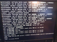
stanleylieber posted a photo: